Qlik Sense Pivot Table – Learn Pivoting in Qlik Sense

Earlier, we discussed Maps in Qlik Sense. Today, we will see the Qlik Sense Pivot Table. In this tutorial, we will learn about a special kind of table known as the pivot table. Also, we will see how different is the pivot table from the normal table and how to use it. 

So, let’s start Qlik Sense Pivot Table.

Qlik Sense Pivot Table – Learn Pivoting in Qlik Sense

1. What is Qlik Sense Pivot Table?

A pivot table consists of rows and columns which contains dimensions and measure fields. We can switch the position of dimensions and measures between columns and rows in a pivot table. We call it pivoting. By pivoting the view of table changes and the field values are shown accordingly. In a pivot table, you can view multiple dimensions and measures interchangeably in different views.

Recommended Reading – Tables in Qlik Sense

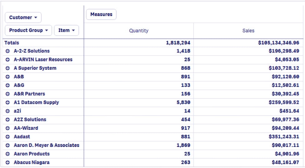
View Multiple Dimensions and Measures

Shown above is a pivot table having three dimensions on the left in the row section and two measures Quantity and Sales on the right section which collectively displays all the measure fields as columns. You move dimensions or measures from column to rows or rows to columns section by dragging them.

For instance, if we move the dimension Customer to the columns section on the right, the table will be updated to show Quantity and Sales for each customer.

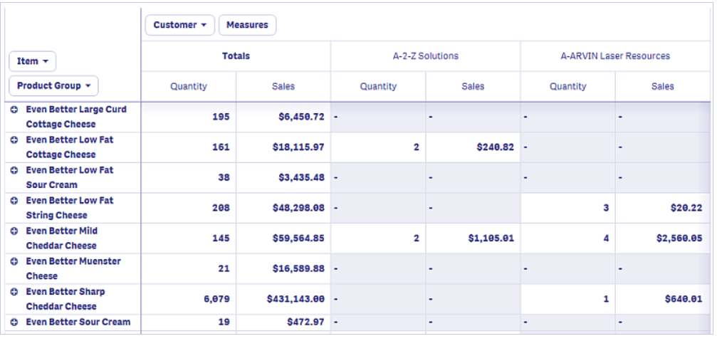
Quantity and sales for each customer

2. How to Create a Qlik Sense Pivot Table?

In order to create a Qlik Sense Pivot Table, follow the steps below.

Step 1: Open the editor of the sheet of the application in which you want to create a pivot table. The editor is opened from the Edit option present on the toolbar of the sheet.

Step 2: Select the option Pivot table (from the Assets Panel) and add it to the editing grid at the center by dragging and dropping.

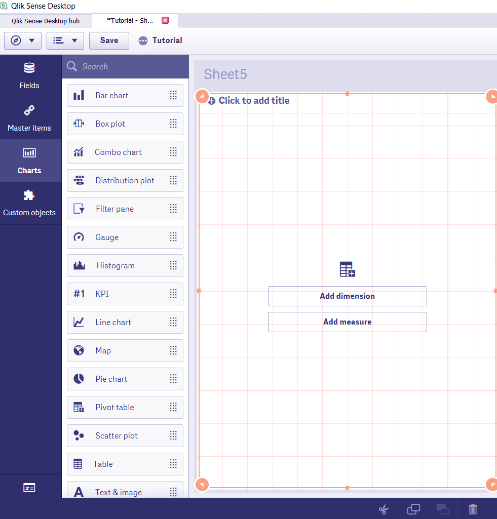
Select Pivot Table from Asserts Panel

Step 3: Add a measure and dimension to start with creating the table. You add more columns in the table from the properties panel at the right of the editor.

Step 4: Once you are done with selecting and adjusting all the aspects of the table from the properties panel, the table will be displayed on the editor instantly. Click Done to bring it on the sheet.

Displaying the Table

3. Properties Panel in Qlik Sense Pivot Table

From the properties panel present at the right of the editor, you can manage different aspects of the pivot table and modify it according to your requirement.

Have a look at Qlik Sense Line Charts

i. Data

From the data tab, you can add dimensions and measures as row and column for the table. You can do the pivoting of dimensions and measures from here also by dragging the field names up and down.  

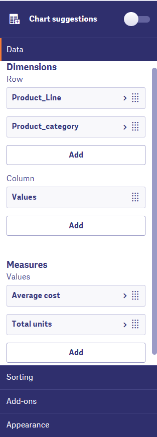
Add Dimensions and Measures

You can edit each column individually by clicking on the arrow given beside the name of the column. The options include expression, label, number formatting (if it is a measure), etc.

ii. Sorting

From the sorting tab you can sort the dimensions and measures in different ways, like sort by the expression, sort by load order, sort numerically, sort alphabetically etc.

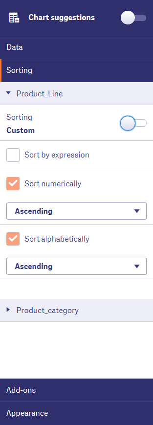
Sorting in Qlik Sense Pivot Table

iii. Add-ons

In this section, you can use the data handling option to apply certain display conditions on the data used in the pivot table. The ‘Include zero values’ option includes all the 0s that are present in a measure field as value and displays them.  

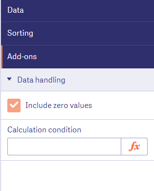
Add-ons section in Qlik Sense

iv. Appearance

The appearance section contains all the setting related to the appearance of the pivot table.  

The first section is the General section has options for showing or hiding titles or details. The Presentation section gives you options to fully expand the table without any collapsed rows and to indent rows.

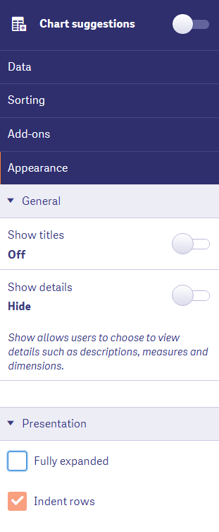
Presentation Section in Qlik Sense Pivot Table

If you do not select the Fully expanded option, then the table will look as shown in the image below.

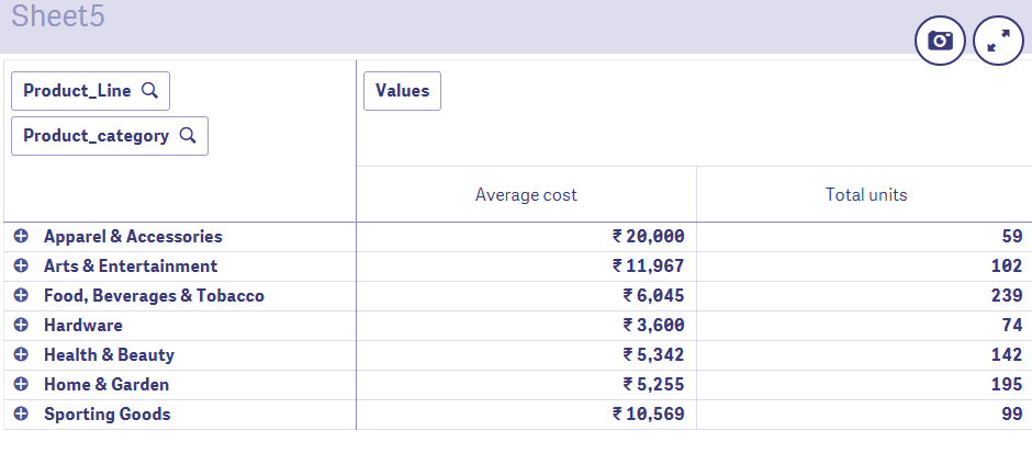
Fully expanded option is not selected

But, if you select the Fully expanded option, then the table is expanded to show all the details and values.

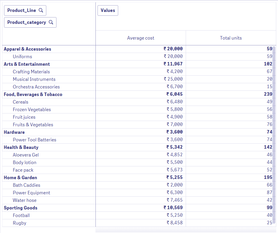
Fully expanded option is selected

Do you know about Qlik Sense Scatter Plot Visualization?

4. Pivoting in Qlik Sense

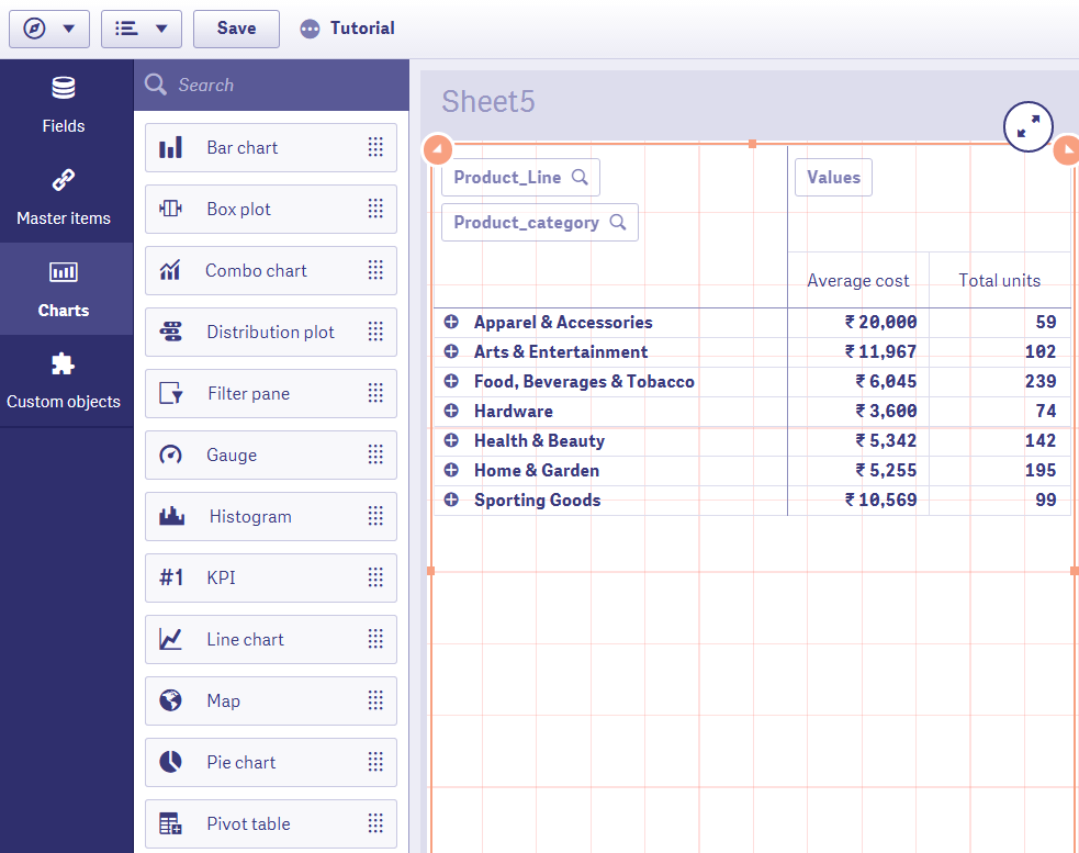
In a Qlik Sense Pivot Table, pivoting can be done in two ways, i.e. either from the properties panel or from the pivot table present on the sheet. Refer to the table that we created in the ‘Creating a pivot table’ section. We can apply pivoting by moving the dimension ‘Product_line’ to the measures/columns section. The updated pivot table is shown in the image below. As you can see, it shows average cost and total units for each product_line like Apparel & Accessories, Arts & Entertainments, Hardware etc. In each of these columns, the values are shown corresponding to the product category values and other cells are left blank with a dash in them.

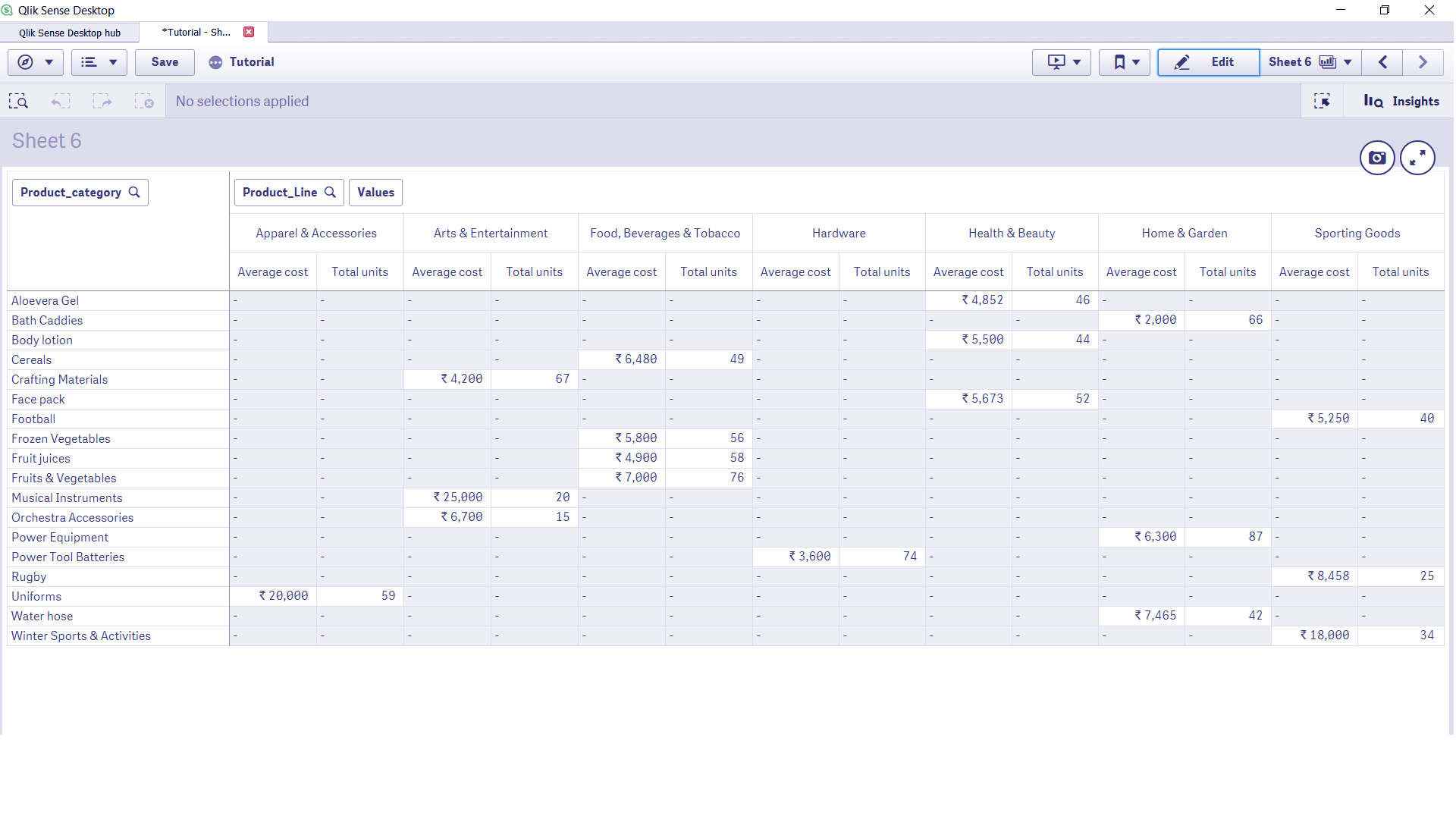
Pivoting in Qlik Sense

You can also apply limitations or conditions on the data set and do global grouping which reflects on all the dimension and measure values. This is done from the data section of the properties panel.

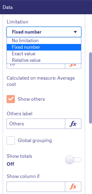
Apply limitations and conditions on the data set

For instance, in the table shown below, which has names of sales representative and year. On the other hand, the column section is the sum(Sales) measure.

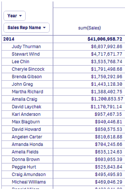
Qlik Sense Pivoting

We will apply limitations on this table such that only those sales representative’s names will be shown which have the top 5 total sales. This limitation or condition will be applied to all the year through global grouping.

Applying limitations on the table

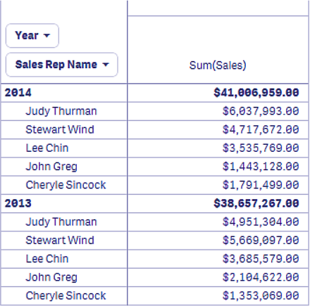
Thus, the new pivot table will only show the top 5 sales representative for each year.

5. Advantages and Limitations

The biggest advantage of using a pivot table is that you can view data in different forms with different perspectives. You can shuffle between rows and columns and dimensions and measures to gain new views of the table. You can use multiple dimensions and measures in pivoting. Although, for some users what comes out as a limitation is that pivot tables might seem complicated to deal with sometimes and requires some skills.

Let’s revise Qlik Sense Logical Functions

So, this was all in Qlik Sense Pivot Table.

6. Conclusion

Thus, this was all that we needed to learn in Qlik Sense Pivot Table. We hope this information helped you in creating a pivot table using your data. Still, if you feel any query related to Qlik Sense Pivot table ask in the comment section. 

You must check – Qlik Sense Financial Functions