8 Machine Learning Algorithms in Python – You Must Learn
Machine Learning courses with 100+ Real-time projects Start Now!!
Master Python with 70+ Hands-on Projects and Get Job-ready - Learn Python
Previously, we discussed the techniques of machine learning with Python. Going deeper, today, we will learn and implement 8 top Machine Learning Algorithms in Python.
Think of these 8 algorithms as the only toolkit for your data. Just like a carpenter knows exactly when to use a hammer or a saw, you’re about to learn and teach our Python scripts, how to actually think, categorize, and forecast like a pro.
Let’s begin the journey of Machine Learning Algorithms in Python Programming.
Machine Learning Algorithms in Python
The following are the Algorithms of Python Machine Learning:
a. Linear Regression in ML
Linear regression is one of the supervised Machine learning algorithms in Python that observes continuous features and predicts an outcome. Depending on whether it runs on a single variable or on many features, we can call it simple linear regression or multiple linear regression.
This is one of the most popular Python ML algorithms and often under-appreciated. It assigns optimal weights to variables to create a line ax+b to predict the output. We often use linear regression to estimate real values like a number of calls and costs of houses based on continuous variables. The regression line is the best line that fits Y=a*X+b to denote a relationship between independent and dependent variables.
Do you know about Python Machine Learning Environment Setup
Let’s plot this for the diabetes dataset.
>>> import matplotlib.pyplot as plt
>>> import numpy as np
>>> from sklearn import datasets,linear_model
>>> from sklearn.metrics import mean_squared_error,r2_score
>>> diabetes=datasets.load_diabetes()
>>> diabetes_X=diabetes.data[:,np.newaxis,2]
>>> diabetes_X_train=diabetes_X[:-30] #splitting data into training and test sets
>>> diabetes_X_test=diabetes_X[-30:]
>>> diabetes_y_train=diabetes.target[:-30] #splitting targets into training and test sets
>>> diabetes_y_test=diabetes.target[-30:]
>>> regr=linear_model.LinearRegression() #Linear regression object
>>> regr.fit(diabetes_X_train,diabetes_y_train) #Use training sets to train the model
LinearRegression(copy_X=True, fit_intercept=True, n_jobs=1, normalize=False)
>>> diabetes_y_pred=regr.predict(diabetes_X_test) #Make predictions
>>> regr.coef_
array([941.43097333])
>>> mean_squared_error(diabetes_y_test,diabetes_y_pred)
3035.0601152912695
>>> r2_score(diabetes_y_test,diabetes_y_pred) #Variance score
0.410920728135835
>>> plt.scatter(diabetes_X_test,diabetes_y_test,color ='lavender')
<matplotlib.collections.PathCollection object at 0x0584FF70>
>>> plt.plot(diabetes_X_test,diabetes_y_pred,color='pink',linewidth=3)
[<matplotlib.lines.Line2D object at 0x0584FF30>]
>>> plt.xticks(())
([], <a list of 0 Text xticklabel objects>)
>>> plt.yticks(())
([], <a list of 0 Text yticklabel objects>)
>>> plt.show()
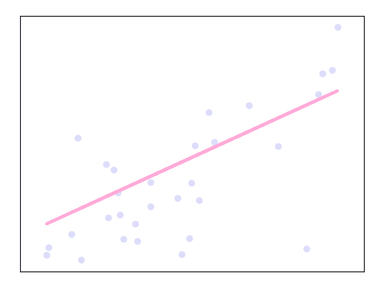
Machine Learning Algorithms in Python – Linear Regression
Python Machine Learning – Data Preprocessing, Analysis & Visualization
b. Logistic Regression in ML
Logistic regression is a supervised classification algorithm unique among Machine Learning algorithms in Python that finds its use in estimating discrete values like 0/1, yes/no, and true/false. This is based on a given set of independent variables. We use a logistic function to predict the probability of an event, and this gives us an output between 0 and 1.
Although it says ‘regression’, this is actually a classification algorithm. Logistic regression fits data into a logit function and is also called logit regression. Let’s plot this.
>>> import numpy as np
>>> import matplotlib.pyplot as plt
>>> from sklearn import linear_model
>>> xmin,xmax=-7,7 #Test set; straight line with Gaussian noise
>>> n_samples=77
>>> np.random.seed(0)
>>> x=np.random.normal(size=n_samples)
>>> y=(x>0).astype(np.float)
>>> x[x>0]*=3
>>> x+=.4*np.random.normal(size=n_samples)
>>> x=x[:,np.newaxis]
>>> clf=linear_model.LogisticRegression(C=1e4) #Classifier
>>> clf.fit(x,y)
>>> plt.figure(1,figsize=(3,4))
<Figure size 300x400 with 0 Axes>
>>> plt.clf()
>>> plt.scatter(x.ravel(),y,color='lavender',zorder=17)
<matplotlib.collections.PathCollection object at 0x057B0E10>
>>> x_test=np.linspace(-7,7,277)
>>> def model(x):
         return 1/(1+np.exp(-x))
>>> loss=model(x_test*clf.coef_+clf.intercept_).ravel()
>>> plt.plot(x_test,loss,color='pink',linewidth=2.5)
[<matplotlib.lines.Line2D object at 0x057BA090>]
>>> ols=linear_model.LinearRegression()
>>> ols.fit(x,y)
LinearRegression(copy_X=True, fit_intercept=True, n_jobs=1, normalize=False)
>>> plt.plot(x_test,ols.coef_*x_test+ols.intercept_,linewidth=1)
[<matplotlib.lines.Line2D object at 0x057BA0B0>]
>>> plt.axhline(.4,color='.4')
<matplotlib.lines.Line2D object at 0x05860E70>
>>> plt.ylabel('y')Text(0,0.5,’y’)
>>> plt.xlabel('x')Text(0.5,0,’x’)
>>> plt.xticks(range(-7,7))
>>> plt.yticks([0,0.4,1])
>>> plt.ylim(-.25,1.25)
(-0.25, 1.25)
>>> plt.xlim(-4,10)
(-4, 10)
>>> plt.legend(('Logistic Regression','Linear Regression'),loc='lower right',fontsize='small')<matplotlib.legend.Legend object at 0x057C89F0>
Do you know how to split the train and Test Set in Python Machine Learning
>>> plt.show()
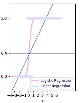
Machine Learning Algorithms in Python -Logistic
c. Decision Tree in ML
A decision tree falls under supervised Machine Learning Algorithms in Python and comes in use for both classification and regression, although mostly for classification. This model takes an instance, traverses the tree, and compares important features with a determined conditional statement. Whether, it descends to the left child branch or the right depends on the result. Usually, more important features are closer to the root.
Decision Tree, a machine learning algorithm in Python, can work on both categorical and continuous dependent variables. Here, we split a population into two or more homogeneous sets. Let’s see the algorithm for this-
>>> from sklearn.cross_validation import train_test_split
>>> from sklearn.tree import DecisionTreeClassifier
>>> from sklearn.metrics import accuracy_score
>>> from sklearn.metrics import classification_report
>>> def importdata(): #Importing data
 balance_data=pd.read_csv('https://archive.ics.uci.edu/ml/machine-learning-'+
'databases/balance-scale/balance-scale.data',
   sep= ',', header = None)
          print(len(balance_data))
          print(balance_data.shape)
          print(balance_data.head())
          return balance_data
>>> def splitdataset(balance_data): #Splitting data
          x=balance_data.values[:,1:5]
          y=balance_data.values[:,0]
          x_train,x_test,y_train,y_test=train_test_split(
              x,y,test_size=0.3,random_state=100)
          return x,y,x_train,x_test,y_train,y_test
>>> def train_using_gini(x_train,x_test,y_train): #Training with giniIndex
          clf_gini = DecisionTreeClassifier(criterion = "gini",
          random_state = 100,max_depth=3, min_samples_leaf=5)
          clf_gini.fit(x_train,y_train)
          return clf_gini
>>> def train_using_entropy(x_train,x_test,y_train): #Training with entropy
          clf_entropy=DecisionTreeClassifier(
          criterion = "entropy", random_state = 100,
          max_depth = 3, min_samples_leaf = 5)
          clf_entropy.fit(x_train,y_train)
          return clf_entropy
>>> def prediction(x_test,clf_object): #Making predictions
          y_pred=clf_object.predict(x_test)
          print(f"Predicted values: {y_pred}")
          return y_pred
>>> def cal_accuracy(y_test,y_pred): #Calculating accuracy
          print(confusion_matrix(y_test,y_pred))
          print(accuracy_score(y_test,y_pred)*100)
          print(classification_report(y_test,y_pred))
>>> data=importdata()
625
(625, 5)
0 1 2 3 4
0 B 1 1 1 1
1 R 1 1 1 2
2 R 1 1 1 3
3 R 1 1 1 4
4 R 1 1 1 5
>>> x,y,x_train,x_test,y_train,y_test=splitdataset(data)
>>> clf_gini=train_using_gini(x_train,x_test,y_train)
>>> clf_entropy=train_using_entropy(x_train,x_test,y_train)
>>> y_pred_gini=prediction(x_test,clf_gini)
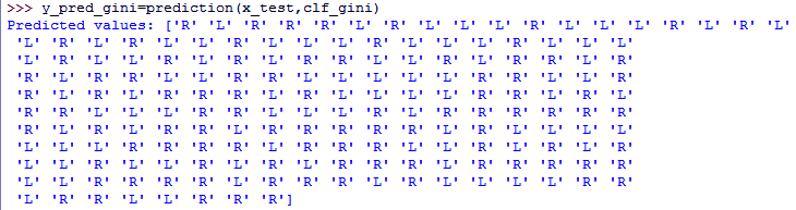
Machine Learning Algorithms in Python – Decision Tree
>>> cal_accuracy(y_test,y_pred_gini)
[[ 0 6 7]
[ 0 67 18]
[ 0 19 71]]
73.40425531914893
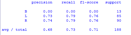
Machine Learning Algorithms in Python – Decision Tree
>>> y_pred_entropy=prediction(x_test,clf_entropy)
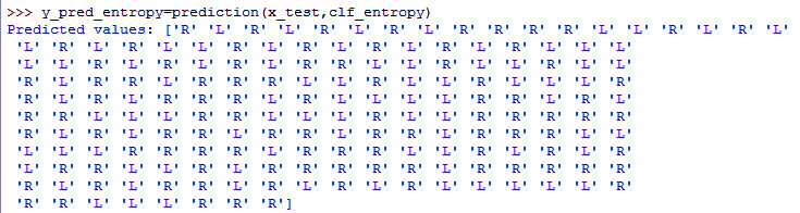
Machine Learning Algorithms in Python – Decision Tree
>>> cal_accuracy(y_test,y_pred_entropy)
[[ 0 6 7]
[ 0 63 22]
[ 0 20 70]]
70.74468085106383

Machine Learning Algorithms in Python – Decision Tree Algorithm i
Let’s explore 4 Machine Learning Techniques with Python
d. Support Vector Machines (SVM) in ML
SVM is a supervised classification algorithm that is one of the most important Machine Learning algorithms in Python, which plots a line that divides different categories of your data. However, in this ML algorithm, we calculate the vector to optimize the line.
This is to ensure that the closest point in each group lies farthest from the others. While you will almost always find this to be a linear vector, it can be other than that.
In this Python Machine Learning tutorial, we plot each data item as a point in an n-dimensional space. We have n features, and each feature has the value of a certain coordinate.
First, let’s plot a dataset.
>>> from sklearn.datasets.samples_generator import make_blobs
>>> x,y=make_blobs(n_samples=500,centers=2,
           random_state=0,cluster_std=0.40)
>>> import matplotlib.pyplot as plt
>>> plt.scatter(x[:,0],x[:,1],c=y,s=50,cmap='plasma')
<matplotlib.collections.PathCollection object at 0x04E1BBF0>
>>> plt.show()
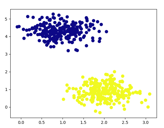
Machine Learning Algorithms in Python – SVM
>>> import numpy as np
>>> xfit=np.linspace(-1,3.5)
>>> plt.scatter(X[:, 0], X[:, 1], c=Y, s=50, cmap='plasma')
<matplotlib.collections.PathCollection object at 0x07318C90>
>>> for m, b, d in [(1, 0.65, 0.33), (0.5, 1.6, 0.55), (-0.2, 2.9, 0.2)]:
        yfit = m * xfit + b
        plt.plot(xfit, yfit, '-k')
        plt.fill_between(xfit, yfit - d, yfit + d, edgecolor='none',
        color='#AFFEDC', alpha=0.4)
[<matplotlib.lines.Line2D object at 0x07318FF0>]
<matplotlib.collections.PolyCollection object at 0x073242D0>
[<matplotlib.lines.Line2D object at 0x07318B70>]
<matplotlib.collections.PolyCollection object at 0x073246F0>
[<matplotlib.lines.Line2D object at 0x07324370>]
<matplotlib.collections.PolyCollection object at 0x07324B30>
>>> plt.xlim(-1,3.5)
(-1, 3.5)
>>> plt.show()
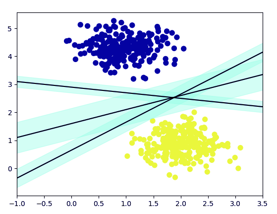
Machine Learning Algorithms in Python – Support Vector Machine
Follow this link to know about Python PyQt5 Tutorial
e. Naive Bayes in ML
Naive Bayes is a classification method that is based on Bayes’ theorem. This assumes independence between predictors. A Naive Bayes classifier will assume that a feature in a class is unrelated to any other. Consider a fruit. This is an apple if it is round, red, and 2.5 inches in diameter. In addition, a Naive Bayes classifier will say these characteristics independently contribute to the probability of the fruit being an apple. This is even if features depend on each other.
Furthermore, for very large data sets, it is easy to build a Naive Bayesian model. Not only is this model very simple, but it also performs better than many highly sophisticated classification methods. Let’s build this.
>>> from sklearn.naive_bayes import GaussianNB
>>> from sklearn.naive_bayes import MultinomialNB
>>> from sklearn import datasets
>>> from sklearn.metrics import confusion_matrix
>>> from sklearn.model_selection import train_test_split
>>> iris=datasets.load_iris()
>>> x=iris.data
>>> y=iris.target
>>> x_train,x_test,y_train,y_test=train_test_split(x,y,test_size=0.3,random_state=0)
>>> gnb=GaussianNB()
>>> mnb=MultinomialNB()
>>> y_pred_gnb=gnb.fit(x_train,y_train).predict(x_test)
>>> cnf_matrix_gnb = confusion_matrix(y_test, y_pred_gnb)
>>> cnf_matrix_gnb
array([[16, 0, 0],
[ 0, 18, 0],
[ 0, 0, 11]], dtype=int64)
>>> y_pred_mnb = mnb.fit(x_train, y_train).predict(x_test)
>>> cnf_matrix_mnb = confusion_matrix(y_test, y_pred_mnb)
>>> cnf_matrix_mnb
array([[16, 0, 0],
[ 0, 0, 18],
[ 0, 0, 11]], dtype=int64)
f. kNN (k-Nearest Neighbors) in ML
This is a Python machine learning algorithm for classification and regression, mostly for classification. This is a supervised learning algorithm that considers different centroids and uses a Euclidean function to compare distances.
Then, it analyzes the results and classifies each point into a group to optimize it to place with all the closest points to it. It classifies new cases using a majority vote of k of its neighbors. Hence, the case it assigns to a class is the one most common among its K nearest neighbors. For this, it uses a distance function.
i. Training and testing on the entire dataset
>>> from sklearn.datasets import load_iris
>>> iris=load_iris()
>>> x=iris.data
>>> y=iris.target
>>> from sklearn.linear_model import LogisticRegression
>>> logreg=LogisticRegression()
>>> logreg.fit(x,y)
LogisticRegression(C=1.0, class_weight=None, dual=False, fit_intercept=True,
intercept_scaling=1, max_iter=100, multi_class=’ovr’, n_jobs=1,
penalty=’l2′, random_state=None, solver=’liblinear’, tol=0.0001,
verbose=0, warm_start=False)
>>> logreg.predict(x)
array([0, 0, 0, 0, 0, 0, 0, 0, 0, 0, 0, 0, 0, 0, 0, 0, 0, 0, 0, 0, 0, 0,
0, 0, 0, 0, 0, 0, 0, 0, 0, 0, 0, 0, 0, 0, 0, 0, 0, 0, 0, 0, 0, 0,
0, 0, 0, 0, 0, 0, 1, 1, 1, 1, 1, 1, 1, 1, 1, 1, 1, 1, 1, 1, 1, 1,
2, 1, 1, 1, 2, 1, 1, 1, 1, 1, 1, 1, 1, 1, 1, 1, 1, 2, 2, 2, 1, 1,
1, 1, 1, 1, 1, 1, 1, 1, 1, 1, 1, 1, 2, 2, 2, 2, 2, 2, 2, 2, 2, 2,
2, 2, 2, 2, 2, 2, 2, 2, 2, 2, 2, 2, 2, 2, 2, 2, 2, 2, 2, 1, 2, 2,
2, 2, 2, 2, 2, 2, 2, 2, 2, 2, 2, 2, 2, 2, 2, 2, 2, 2])
>>> y_pred=logreg.predict(x)
>>> len(y_pred)
150
>>> from sklearn import metrics
>>> metrics.accuracy_score(y,y_pred)
0.96
>>> from sklearn.neighbors import KNeighborsClassifier
>>> knn=KNeighborsClassifier(n_neighbors=5)
>>> knn.fit(x,y)
KNeighborsClassifier(algorithm=’auto’, leaf_size=30, metric=’minkowski’,
metric_params=None, n_jobs=1, n_neighbors=5, p=2,
weights=’uniform’)
>>> y_pred=knn.predict(x)
>>> metrics.accuracy_score(y,y_pred)
0.9666666666666667
>>> knn=KNeighborsClassifier(n_neighbors=1)
>>> knn.fit(x,y)
KNeighborsClassifier(algorithm=’auto’, leaf_size=30, metric=’minkowski’,
metric_params=None, n_jobs=1, n_neighbors=1, p=2,
weights=’uniform’)
>>> y_pred=knn.predict(x)
>>> metrics.accuracy_score(y,y_pred)
1.0
ii. Splitting into train/test
>>> x.shape
(150, 4)
>>> y.shape
(150,)
>>> from sklearn.cross_validation import train_test_split
>>> x.shape
(150, 4)
>>> y.shape
(150,)
>>> from sklearn.cross_validation import train_test_split
>>> x_train,x_test,y_train,y_test=train_test_split(x,y,test_size=0.4,random_state=4)
>>> x_train.shape
(90, 4)
>>> x_test.shape
(60, 4)
>>> y_train.shape
(90,)
>>> y_test.shape
(60,)
>>> logreg=LogisticRegression()
>>> logreg.fit(x_train,y_train)
>>> y_pred=knn.predict(x_test)
>>> metrics.accuracy_score(y_test,y_pred)
0.9666666666666667
>>> knn=KNeighborsClassifier(n_neighbors=5)
>>> knn.fit(x_train,y_train)
KNeighborsClassifier(algorithm=’auto’, leaf_size=30, metric=’minkowski’,
metric_params=None, n_jobs=1, n_neighbors=5, p=2,
weights=’uniform’)
>>> y_pred=knn.predict(x_test)
>>> metrics.accuracy_score(y_test,y_pred)
0.9666666666666667
>>> k_range=range(1,26)
>>> scores=[]
>>> for k in k_range:
         knn = KNeighborsClassifier(n_neighbors=k)
         knn.fit(x_train, y_train)
         y_pred = knn.predict(x_test)
         scores.append(metrics.accuracy_score(y_test, y_pred))
>>> scores
[0.95, 0.95, 0.9666666666666667, 0.9666666666666667, 0.9666666666666667, 0.9833333333333333, 0.9833333333333333, 0.9833333333333333, 0.9833333333333333, 0.9833333333333333, 0.9833333333333333, 0.9833333333333333, 0.9833333333333333, 0.9833333333333333, 0.9833333333333333, 0.9833333333333333, 0.9833333333333333, 0.9666666666666667, 0.9833333333333333, 0.9666666666666667, 0.9666666666666667, 0.9666666666666667, 0.9666666666666667, 0.95, 0.95]
>>> import matplotlib.pyplot as plt
>>> plt.plot(k_range,scores)
[<matplotlib.lines.Line2D object at 0x05FDECD0>]
>>> plt.xlabel('k for kNN')Text(0.5,0,’k for kNN’)
>>> plt.ylabel('Testing Accuracy')Text(0,0.5,’Testing Accuracy’)
>>> plt.show()
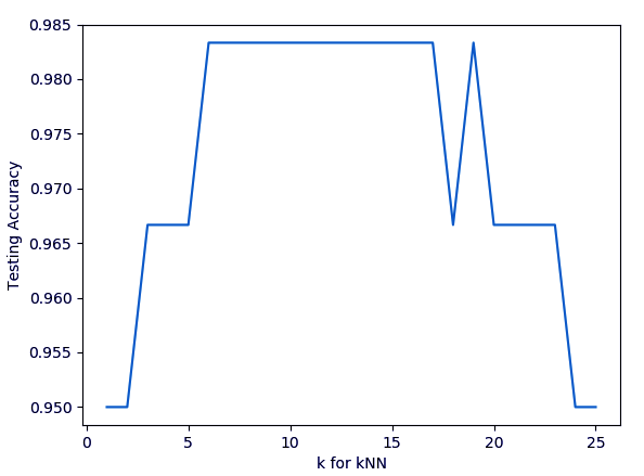
Machine Learning Algorithms in Python – k-Nearest Neighbors
Read about Python Statistics – p-Value, Correlation, T-test, KS Test
g. k-Means in ML
k-Means is an unsupervised algorithm that solves the problem of clustering. It classifies data using several clusters. The data points inside a class are homogeneous and heterogeneous to peer groups.
>>> import numpy as np
>>> import matplotlib.pyplot as plt
>>> from matplotlib import style
>>> style.use('ggplot')
>>> from sklearn.cluster import KMeans
>>> x=[1,5,1.5,8,1,9]
>>> y=[2,8,1.7,6,0.2,12]
>>> plt.scatter(x,y)
<matplotlib.collections.PathCollection object at 0x0642AF30>
>>> x=np.array([[1,2],[5,8],[1.5,1.8],[8,8],[1,0.6],[9,11]])
>>> kmeans=KMeans(n_clusters=2)
>>> kmeans.fit(x)
KMeans(algorithm=’auto’, copy_x=True, init=’k-means++’, max_iter=300,
n_clusters=2, n_init=10, n_jobs=1, precompute_distances=’auto’,
random_state=None, tol=0.0001, verbose=0)
>>> centroids=kmeans.cluster_centers_
>>> labels=kmeans.labels_
>>> centroids
array([[1.16666667, 1.46666667],
[7.33333333, 9. ]])
>>> labels
array([0, 1, 0, 1, 0, 1])
>>> colors=['g.','r.','c.','y.']
>>> for i in range(len(x)):
         print(x[i],labels[i])
         plt.plot(x[i][0],x[i][1],colors[labels[i]],markersize=10)
[1. 2.] 0
[<matplotlib.lines.Line2D object at 0x0642AE10>]
[5. 8.] 1
[<matplotlib.lines.Line2D object at 0x06438930>]
[1.5 1.8] 0
[<matplotlib.lines.Line2D object at 0x06438BF0>]
[8. 8.] 1
[<matplotlib.lines.Line2D object at 0x06438EB0>]
[1. 0.6] 0
[<matplotlib.lines.Line2D object at 0x06438FB0>]
[ 9. 11.] 1
[<matplotlib.lines.Line2D object at 0x043B1410>]
>>> plt.scatter(centroids[:,0],centroids[:,1],marker='x',s=150,linewidths=5,zorder=10)
<matplotlib.collections.PathCollection object at 0x043B14D0>
>>> plt.show()
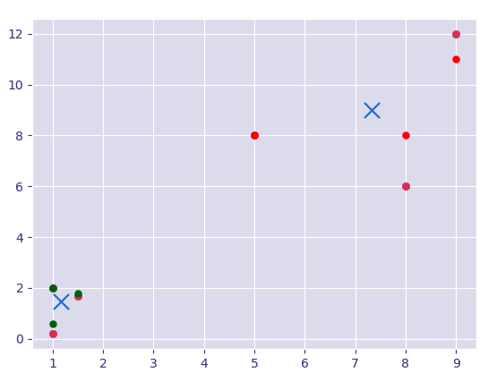
Machine Learning Algorithms in Python – K-Means
Have a Look at Python Descriptive Statistics – Measuring Central Tendency
h. Random Forest in ML
A random forest is an ensemble of decision trees. Now, to classify every new object based on its attributes, trees vote for a class- each tree provides a classification. The classification with the most votes wins in the forest.
>>> import numpy as np
>>> import pylab as pl
>>> x=np.random.uniform(1,100,1000)
>>> y=np.log(x)+np.random.normal(0,.3,1000)
>>> pl.scatter(x,y,s=1,label='log(x) with noise')
<matplotlib.collections.PathCollection object at 0x0434EC50>
>>> pl.plot(np.arange(1,100),np.log(np.arange(1,100)),c='b',label='log(x) true function')
[<matplotlib.lines.Line2D object at 0x0434EB30>]
>>> pl.xlabel('x')Text(0.5,0,’x’)
>>> pl.ylabel('f(x)=log(x)')Text(0,0.5,’f(x)=log(x)’)
>>> pl.legend(loc='best')
<matplotlib.legend.Legend object at 0x04386450>
>>> pl.title('A basic log function')
Text(0.5,1,’A basic log function’)
>>> pl.show()
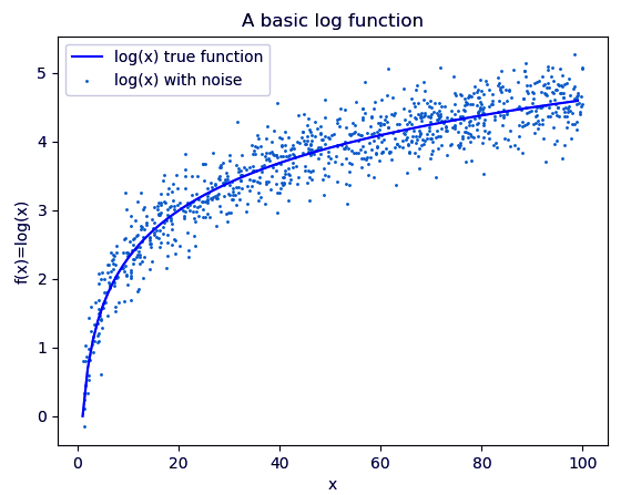
Machine Learning Algorithms in Python – Random Forest
>>> from sklearn.datasets import load_iris
>>> from sklearn.ensemble import RandomForestClassifier
>>> import pandas as pd
>>> import numpy as np
>>> iris=load_iris()
>>> df=pd.DataFrame(iris.data,columns=iris.feature_names)
>>> df['is_train']=np.random.uniform(0,1,len(df))<=.75
>>> df['species']=pd.Categorical.from_codes(iris.target,iris.target_names)
>>> df.head()
sepal length (cm) sepal width (cm) … is_train species
0 5.1 3.5 … True setosa
1 4.9 3.0 … True setosa
2 4.7 3.2 … True setosa
3 4.6 3.1 … True setosa
4 5.0 3.6 … False setosa
[5 rows x 6 columns]
>>> train,test=df[df['is_train']==True],df[df['is_train']==False]
>>> features=df.columns[:4]
>>> clf=RandomForestClassifier(n_jobs=2)
>>> y,_=pd.factorize(train['species'])
>>> clf.fit(train[features],y)
RandomForestClassifier(bootstrap=True, class_weight=None, criterion=’gini’,
max_depth=None, max_features=’auto’, max_leaf_nodes=None,
min_impurity_decrease=0.0, min_impurity_split=None,
min_samples_leaf=1, min_samples_split=2,
min_weight_fraction_leaf=0.0, n_estimators=10, n_jobs=2,
oob_score=False, random_state=None, verbose=0,
warm_start=False)
>>> preds=iris.target_names[clf.predict(test[features])]
>>> pd.crosstab(test['species'],preds,rownames=['actual'],colnames=['preds'])
preds setosa versicolor virginica
actual
setosa 12 0 0
versicolor 0 17 2
virginica 0 1 15
Other important techniques in AI are deep learning, which includes convolutional neural networks (CNNs) and recurrent neural networks (RNNs).
These algorithms make up some of the modern preferences that include image and speech recognition, natural language processing, and others. Still, the conventional methods of machine learning, like the ones discussed here, are basic, and deep learning methods have added possibilities and are used in the contemporary methodologies of machine learning and AI.
So, this was all about Machine Learning Algorithms in Python Tutorial. Hope you like our explanation.
Conclusion
Python has many ready-to-use machine learning algorithms. These are like recipes for solving problems. Some popular ones are Linear Regression, Decision Tree, Random Forest, Support Vector Machine (SVM), K-Nearest Neighbors (KNN), and Naive Bayes. Each algorithm works in a different way and fits different types of problems.
For example, Linear Regression is good for predicting numbers, like sales or prices. Decision Trees are easy to understand and great for yes/no problems. Random Forest is a powerful version of decision trees that reduces errors.
As a result, SVM is strong when there is a clear gap between classes. KNN is simple and works by comparing new data to old data. Naive Bayes is often used for spam detection or sentiment analysis.
Did you like our efforts? If Yes, please give DataFlair 5 Stars on Google


Cluster vs classifier
what is the meaning of this line
“matplotlib.collections.PathCollection object at 0x057B0E10”
Scatter plots uses dots or specifies objects to represent realationship between variables. And the scatter method is used to draw scatter plots. So these are just confirming that you have used the scatter methos correctly and now you can draw the plot using plt.show() to get the result.