Python Linear Regression | Chi-Square Test In Python

1. Python Linear Regression – Object

Today, in this Python tutorial, we will discuss Python Linear Regression and Chi-Square Test in Python. Moreover, we will understand the meaning of Linear Regression and Chi-Square in Python. Also, we will look at Python Linear Regression Example and Chi-square example.

So, let’s start with Python Linear Regression.

Python Linear Regression | Chi-Square Test In Python

2. Python Linear Regression

Linear regression is a way to model the relationship that a scalar response(a dependent variable) has with explanatory variable(s)(independent variables). Depending on whether we have one or more explanatory variables, we term it simple linear regression and multiple linear regression in Python.

Do you know about Python SciPy

To model relationships, we use linear predictor functions with unknown model parameters; we call these linear models in Python.

We will use Seaborn to plot a Python linear regression here.

a. Python Linear Regression Example

Let’s take a simple example of Python Linear Regression.

>>> import seaborn as sn
>>> import matplotlib.pyplot as plt
>>> sn.set(color_codes=True)
>>> tips=sn.load_dataset('tips')
>>> ax=sn.regplot(x='total_bill',y='tip',data=tips)
>>> plt.show()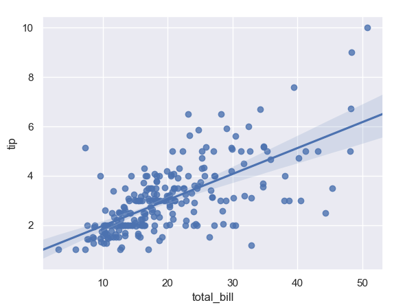

Python Linear Regression Example

b. How to Customize the Color in Python Linear Regression?

Now let’s color it green.
Have a look at Python NumPy

>>> import numpy as np
>>> np.random.seed(7)
>>> mean,cov=[3,5],[(1.3,.8),(.8,1.1)]
>>> x,y=np.random.multivariate_normal(mean,cov,77).T
>>> ax=sn.regplot(x=x,y=y,color='g')
>>> plt.show()

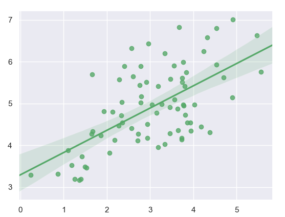
Customizing the colour in Linear regression in Python Programming Language

c. Plotting with Pandas Series, Customizing Markers

Now, we’ll use two Python Pandas Series to plot Python linear regression.

>>> import pandas as pd
>>> x,y=pd.Series(x,name='x'),pd.Series(y,name='y')
>>> ax=sn.regplot(x=x,y=y,marker='*')

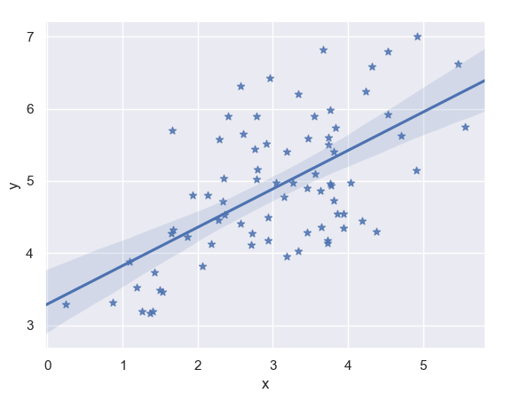
Customizing the color in Python Linear regression

d. Setting a Confidence Interval

To set the confidence interval, we use the ci parameter. The confidence interval is a range of values that make it probable that a parameter’s value lies within it.
Let’s discuss Python Heatmap

>>> ax=sn.regplot(x=x,y=y,ci=68)
>>> plt.show()

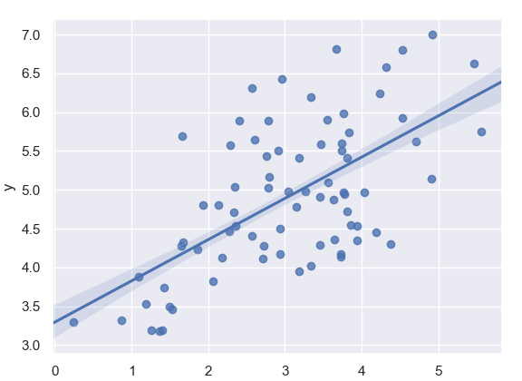
Setting a Confidence Interval

e. Adding Jitter

You can add some jitter in the x or y directions.

>>> ax=sn.regplot(x='size',y='total_bill',data=tips,y_jitter=.1,color='g')
>>> plt.show()

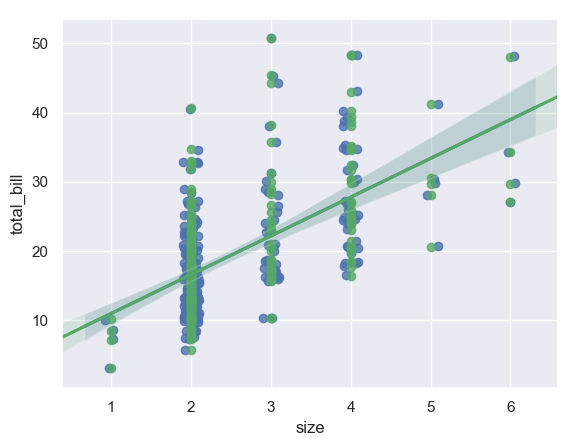
Adding Jitter in Python Linear Regression

f. Plotting With a Continuous Variable Divided into Discrete Bins

Let’s revise the Python Charts
Let’s create 5 bins and make the plot.

>>> ax=sn.regplot(x=x,y=y,x_bins=5)
>>> plt.show()

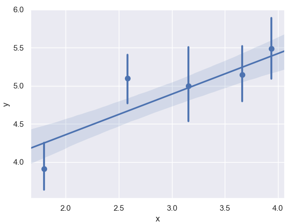
Plotting With a Continuous Variable Divided into Discrete Bins

3. What is the Chi-Square Test?

This is a statistical hypothesis test that uses a chi-squared distribution as a sampling distribution for the test statistic when we have a true null hypothesis. In other words, it is a way to assess how a set of observed values fits in with the values expected in theory- the goodness of fit.
You must know about Python Data Science
The test tells us whether, in one or more categories, the expected frequencies differ significantly from the observed frequencies. We also write it as χ2 test. In this test, we classify observations into mutually exclusive classes. A null hypothesis tells us how probable it is that an observation falls into the corresponding class. With this test, we aim to determine how likely an observation made is, while assuming that the null hypothesis is true. This Chi-Square test tells us whether two categorical variables depend on each other.

a. Python Chi-Square Example

Let’s take an example.

>>> from scipy import stats
>>> import numpy as np
>>> import matplotlib.pyplot as plt
>>> x=np.linspace(0,10,100)
>>> fig,ax=plt.subplots(1,1)
>>> linestyles=['--','-.',':','-']
>>> degrees_of_freedom=[1,3,7,5]
>>> for df,ls in zip(degrees_of_freedom,linestyles):
                ax.plot(x,stats.chi2.pdf(x,df),linestyle=ls)               

[<matplotlib.lines.Line2D object at 0x060314D0>]
[<matplotlib.lines.Line2D object at 0x06031590>]
[<matplotlib.lines.Line2D object at 0x060318B0>]
[<matplotlib.lines.Line2D object at 0x06031B50>]

>>> plt.xlim(0,7)

(0, 7)

>>> plt.ylim(0,0.5)

(0, 0.5)
Let’s discuss Python Compilers

>>> plt.show()

This code plots four line plots for us-

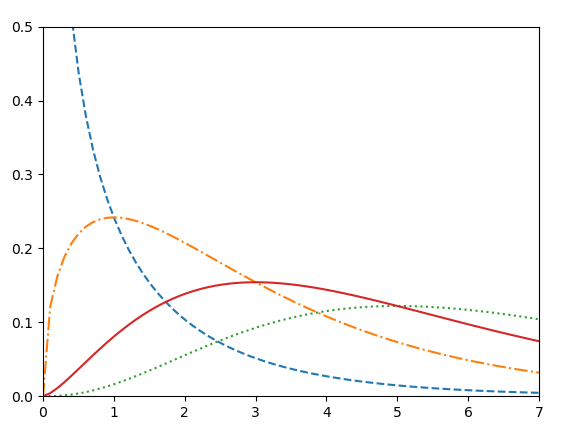
Python Chi-Square Example

b. scipy.stats.chisquare

This calculates a one-way chi-square test for us. It has the following syntax-

scipy.stats.chisquare(f_obs,f_exp=None,ddof=0,axis=0)

Consider the null hypothesis that the categorical data in question has the given frequencies. The Chi-square test tests this.
It has the following parameters-

• f_obs: array_like- In this, we specify the observed frequencies in every category
• f_exp: array_like, optional- This holds the expected frequencies in every category; each category is equally likely by default
• ddof: int, optional- This holds the adjustment value to the degrees of freedom for the p-value
• axis: int or None, optional- This is the axis of the broadcast result of f_obs and f_exp; we apply the test along with this

It has the following return values-

• chisq: float or ndarray- This is the chi-squared test statistic
• p: float or ndarray- This is the p-value of the test

Do you know about Python Geographic maps
This is the formula for the chi-square statistic-
sum((observed-expected)2/expected)

c. Examples of scipy.stats.chisquare

Let’s take a few simple examples.

>>> from scipy.stats import chisquare
>>> chisquare([6,8,6,4,2,2])

Power_divergenceResult(statistic=6.285714285714286, pvalue=0.27940194154949133)

• Providing expected frequencies

>>> chisquare([6,8,6,4,2,2],f_exp=[6,6,6,6,6,8])

Power_divergenceResult(statistic=8.5, pvalue=0.13074778927442537)

• 2D observed frequencies

>>> data=np.array([[6,8,6,4,2,2],[12,10,6,11,10,12]]).T
>>> chisquare(data)

Power_divergenceResult(statistic=array([6.28571429, 2.44262295]), pvalue=array([0.27940194, 0.78511028]))

• Setting axis to None

>>> chisquare(np.array([[6,8,6,4,2,2],[12,8,6,10,7,8]]),axis=None)

Power_divergenceResult(statistic=14.72151898734177, pvalue=0.1956041745113551)
Learn Python Scatter Plot

>>> chisquare(np.array([[6,8,6,4,2,2],[12,8,6,10,7,8]]).ravel())

Power_divergenceResult(statistic=14.72151898734177, pvalue=0.1956041745113551)

• Altering the degrees of freedom

>>> chisquare([6,8,6,4,2,2],ddof=1)

Power_divergenceResult(statistic=6.285714285714286, pvalue=0.17880285265458937)

• Calculating p-values by broadcasting the chi-squared statistic with ddof

>>> chisquare([6,8,6,4,2,2],ddof=[0,1,2])

Power_divergenceResult(statistic=6.285714285714286, pvalue=array([0.27940194, 0.17880285, 0.09850749]))

So, this was all in Python Linear Regression. Hope you like our explanation of Python Chi-Square Test.

4. Conclusion

Hence, in this Python Statistics tutorial, we discussed Python Linear Regression and Python Chi-Square Test. Moreover, we saw the example of Python Linear Regression and chi-square test. Still, if any doubt regarding Python Linear Regression, ask in the comment tab.
See also –
Python Matplotlib
For reference