Probability Distributions in Python – Normal, Binomial, Poisson, Bernoulli
Master Python with 70+ Hands-on Projects and Get Job-ready - Learn Python
After studying Python Descriptive Statistics, now we are going to explore 4 Major Python Probability Distributions: Normal, Binomial, Poisson, and Bernoulli Distributions in Python. Moreover, we will learn how to implement these Python probability distributions with Python Programming.
What is Python Probability Distribution?
A probability distribution is a function under probability theory and statistics- one that gives us how probable different outcomes are in an experiment. It describes events in terms of their probabilities; this is out of all possible outcomes. Let’s take the probability distribution of a fair coin toss. Here, heads take a value of X=0.5, and tails get X=0.5 too.
Two classes of such a distribution are discrete and continuous. The former is represented by a probability mass function and the latter by a probability density function.
Why is probability distribution important?
- It helps in understanding how the data behaves.
- It is also used in statistics, like the p-value.
- It helps in making predictions easier and identifying outliers.Do you know about Python Namedtuple?
How to Implement Python Probability Distributions?
Let’s implement these types of Python Probability Distributions, let’s see them:
a. Normal Distribution in Python
Python normal distribution is a function that distributes random variables in a graph that is shaped as a symmetrical bell. It does so by arranging the probability distribution for each value. Let’s use Python numpy for this.
>>> import scipy.stats
>>> import numpy as np
>>> import matplotlib.pyplot as plt
>>> np.random.seed(1234)
>>> samples=np.random.lognormal(mean=1.,sigma=.4,size=10000)
>>> shape,loc,scale=scipy.stats.lognorm.fit(samples,floc=0)
>>> num_bins=50
>>> clr="#EFEFEF"
>>> counts,edges,patches=plt.hist(samples,bins=num_bins,color=clr)
>>> centers=0.5*(edges[:-1]+edges[1:])
>>> cdf=scipy.stats.lognorm.cdf(edges,shape,loc=loc,scale=scale)
>>> prob=np.diff(cdf)
>>> plt.plot(centers,samples.size*prob,'k-',linewidth=2)
[<matplotlib.lines.Line2D object at 0x0359E890>]
>>> plt.show()
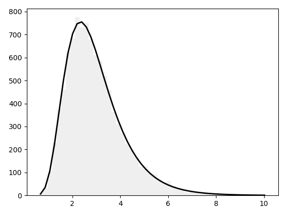
Implement Python Probability Distributions – Normal Distribution in Python
b. Binomial Distribution in Python
Python binomial distribution tells us the probability of how often there will be a success in n independent experiments. Such experiments are yes-no questions. One example may be tossing a coin.
Let’s explore SciPy Tutorial – Linear Algebra, Benefits, Special Functions
>>> import seaborn
>>> from scipy.stats import binom
>>> data=binom.rvs(n=17,p=0.7,loc=0,size=1010)
>>> ax=seaborn.distplot(data,
                kde=True,
                color='pink',
                hist_kws={"linewidth": 22,'alpha':0.77})
>>> ax.set(xlabel='Binomial',ylabel='Frequency')
[Text(0,0.5,’Frequency’), Text(0.5,0,’Binomial’)]
>>> plt.show()
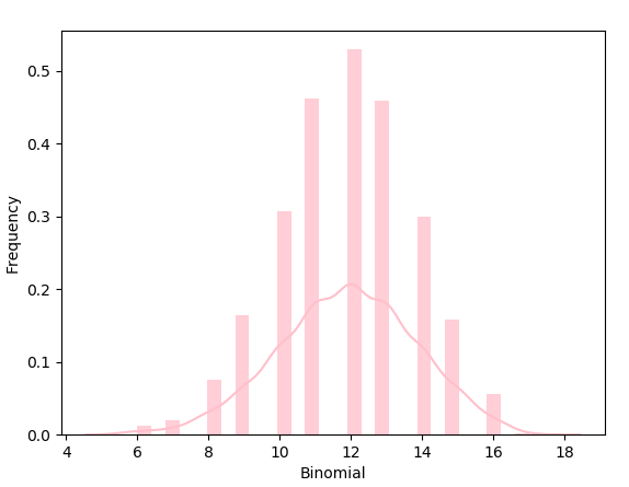
Implement Python Probability Distributions – Binomial Distribution in Python
c. Poisson Distribution in Python
Python Poisson distribution tells us about how probable it is that a certain number of events happen in a fixed interval of time or space. This assumes that these events happen at a constant rate and are also independent of the last event.
>>> import numpy as np
>>> s=np.random.poisson(5, 10000)
>>> import matplotlib.pyplot as plt
>>> plt.hist(s,16,normed=True,color='Green')
(array([5.86666667e-03, 3.55200000e-02, 8.86400000e-02, 1.48906667e-01,
1.91573333e-01, 1.81440000e-01, 1.56160000e-01, 1.16586667e-01,
6.65600000e-02, 3.90400000e-02, 2.06933333e-02, 9.06666667e-03,
3.84000000e-03, 2.13333333e-03, 5.33333333e-04, 1.06666667e-04]), array([ 0. , 0.9375, 1.875 , 2.8125, 3.75 , 4.6875, 5.625 ,
6.5625, 7.5 , 8.4375, 9.375 , 10.3125, 11.25 , 12.1875,
13.125 , 14.0625, 15. ]), <a list of 16 Patch objects>)
Read about What is Python Interpreter – Environment, Invoking & Working
>>> plt.show()
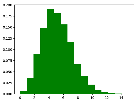
Implement Python Probability Distributions – Poisson Distribution in Python
d. Bernoulli Distribution in Python
Python Bernoulli Distribution is a case of binomial distribution where we conduct a single experiment. This is a discrete probability distribution with probability p for value 1 and probability q=1-p for value 0. p can be for success, yes, true, or one. Similarly, q=1-p can be for failure, no, false, or zero.
>>> s=np.random.binomial(10,0.5,1000)
>>> plt.hist(s,16,normed=True,color='Brown')
(array([0.00177778, 0.02311111, 0. , 0.08711111, 0. ,
0.18666667, 0. , 0.33777778, 0.45155556, 0. ,
0.37688889, 0. , 0.224 , 0. , 0.07466667,
0.01422222]), array([0. , 0.5625, 1.125 , 1.6875, 2.25 , 2.8125, 3.375 , 3.9375,
4.5 , 5.0625, 5.625 , 6.1875, 6.75 , 7.3125, 7.875 , 8.4375,
9. ]), <a list of 16 Patch objects>)
Do you know about Python Django Tutorial For Beginners
>>> plt.show()
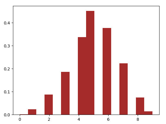
Implement Python Probability Distributions – Bernoulli Distribution in Python
So, this was all about Python Probability Distribution. Hope you like our explanation.
Conclusion
Hence, we studied Python Probability Distribution and its 4 types with an example. In addition, we learned how to implement these Python probability distributions. Furthermore, if you have any doubts, feel free to ask in the comments section.
The normal distribution is the most common and appears as a bell curve. It is symmetric and centered around the mean. Many natural phenomena, like height, test scores, or errors in measurements, follow this distribution
The binomial distribution models the number of successes in a fixed number of independent experiments. It is useful in scenarios like predicting the number of defective items in a batch or the number of heads in coin tosses. Python allows you to model this using binom.pmf() or generate samples using numpy.random.binomial(). The Poisson distribution is used to model the number of events occurring in a fixed interval of time or space, such as the number of calls to a help center.
The Bernoulli distribution is the simplest, dealing with binary outcomes—success or failure, yes or no. It is the basis for logistic regression and classification tasks in machine learning.
Related Topic- How to Work with Relational Database
For reference
Did you like our efforts? If Yes, please give DataFlair 5 Stars on Google


