Python SciPy Tutorial – What is SciPy & How to Install SciPy

In our previous Python Library tutorial, we saw Python Matplotlib. Today, we bring you a tutorial on Python SciPy.

Here in this SciPy Tutorial, we will learn the benefits of Linear Algebra, Working of Polynomials, and how to install SciPy.

Moreover, we will cover the Processing Signals with SciPy, and Processing Images with SciPy.

So, let’s start the Python SciPy Tutorial.

Python SciPy Tutorial – Linear Algebra, Benefits, Special Functions

What is SciPy in Python?

Python SciPy is open-source and BSD-licensed. You can pronounce it as Sigh Pie. Here are some shorts on it:

• Author: Travis Oliphant, Pearu Peterson, Eric Jones.
• First Release: 2001
• Stable Release: Version 1.1.0; May, 2018.
• Written in: Fortran, C, C++, Python Programming Language.

Python SciPy has modules for the following tasks:

• Optimization
• Linear algebra
• Integration
• Interpolation
• Special functions
• FFT
• Signal and Image processing
• ODE solvers

And as we’ve seen, an important feature of the NumPy module is multidimensional arrays.

This is what SciPy uses too; it will work with NumPy arrays.

SciPy Subpackages

In this Python SciPy Tutorial, we will study these following sub-packages of SciPy:

• cluster- Hierarchical clustering.
• constants- Physical constants and factors of conversion.
• fftpack- Algorithms for Discrete Fourier Transform.
• integrate- Routines for numerical integration.
• interpolate- Tools for interpolation.
• io- Input and Output tools for data.
• lib- Wrappers to external libraries.
• linalg- Routines for linear algebra.
• misc- Miscellaneous utilities like image reading and writing.
• ndimage- Functions for processing multidimensional images.
• optimize- Algorithms for optimization.
• signal- Tools for processing signal.
• sparse- Algorithms for sparse matrices.
• spatial- KD-trees, distance functions, nearest neighbors.
• special- Special functions.
• stats- Functions to perform statistics.
• weave- Functionality that lets you write C++/C code in the form of multiline strings.

Benefits of SciPy

• High-level commands and classes for visualizing and manipulating data.
• Powerful and interactive sessions with Python.
• Classes, and web and database routines for parallel programming.
• Easy and fast.
• Open-source.

How to Install SciPy?

You can use pip to install SciPy-

pip install scipy

You can also use conda for the same-

conda install –c anaconda scipy

Then, you can import SciPy as:

>>> import scipy

You will also want to interact with numpy here. Let’s import that too.

>>> import numpy

Finally, in some places, we will want to plot our results. We will use matplotlib for that; let’s import it.

>>> import matplotlib

Linear Algebra in SciPy

For performing operations of linear algebra in SciPy, we will need to import linalg from scipy-

>>> from scipy import linalg

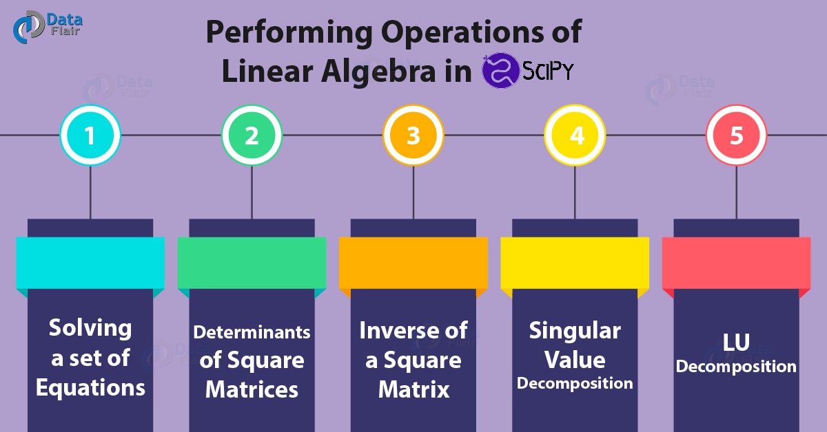
SciPy Tutorial – Linear Algebra

1. Solving a set of equations

Let’s suppose this is the set of equations we want to solve-
2x+3y=7
3x+4y=10
Let’s create input and solution arrays for this.

>>> A=numpy.array([[2,3],[3,4]])
>>> B=numpy.array([[7],[10]])
>>> linalg.solve(A,B)

Output

This tells us that both equations work for x=2 and y=1. To check the results, we run the following command-

>>> A.dot(linalg.solve(A,B))-B

Output

The output confirms the correctness of the computation.

2. Determinants of Square Matrices

To calculate the determinant for a square matrix, we can use the det() method.

>>>mat=numpy.array([[8,2],[1,4]])
>>>linalg.det(mat)

Output

3. An inverse of a Square Matrix

For this, we use the inv() method.

>>> linalg.inv(mat)

Output

4. Singular Value Decomposition

This uses the method svd().

>>> linalg.svd(mat)

Output

5. LU Decomposition

To carry out LU decomposition, we can use the lu() method.

>>> linalg.lu(mat)

Output

Working with Polynomials in SciPy

SciPy will let us work with polynomials using the poly1d type from numpy:

>>> from numpy import poly1d
>>> p=poly1d([3,2,4])

Output

>>> p*p

Output

>>> p(5) #Value of polynomial for x=5

Output

>>> p.integ(k=6) #Integration

Output

>>> p.deriv() #Finding derivatives

Output

Integration with SciPy

To be able to perform integration, we will import the integrate subpackage from scipy.

>>> from scipy import integrate

The quad() function will let us integrate a function; let’s use a lambda for this.

>>> integrate.quad(lambda x:x**2,0,4) #Last two arguments are lower and upper limits

Output

You can use help() function to find out what else this subpackage can do for you. Here are some more functions:

• dblquad- Double integration
• tplquad- Triple integration
• nquad- n-dimensional integration
• fixed_quad- Use Gaussian quadrature of order n to integrate func(x)
• quadrature- Use Gaussian quadrature to integrate with certain tolerance
• romberg- Romberg integration
• quad_explain- Find out about quad
• newton_cotes- Weights and coefficient of error with Newton-Cotes integration
• IntegrationWarning- Warning for issues in integration

Vectorizing Functions in SciPy

The class vectorizes will let us turn a regular Python function into a vectorized function. Let’s try this out.

We’ll define a function first. If the first argument is greater than the second, it returns the sum of the two.

Otherwise, it returns the product of the two.

def addmul(a,b):
         if a>b:
             return a+b
else:
             return a*b

Now, let’s vectorize this.

>>> numpy.vectorize(addmul)([1,4,3,9],[2,3,7,8])

Output

Fast Fourier Transforms in SciPy

If you’re familiar with calculus, then there are chances are you may be familiar with Fourier Transforms.

This analysis lets you express a function as a sum of periodic components. It is possible to recover the signal from this sum.

Let’s take an example.

>>> from scipy.fftpack import fft
>>> N=600
>>> T=1.0/800.0
>>> x=np.linspace(0.0,N*T,N)
>>> y=numpy.sin(50.0*2.0*numpy.pi*x)+0.5*numpy.sin(80.0*2.0*numpy.pi*x)
>>> yf=fft(y)
>>> xf=numpy.linspace(0.0,1.0/(2.0*T),N//2)
>>> import matplotlib.pyplot as plt
>>> plt.plot(xf, 2.0/N * numpy.abs(yf[0:N//2]))

Output

>>> plt.grid()
>>> plt.show()

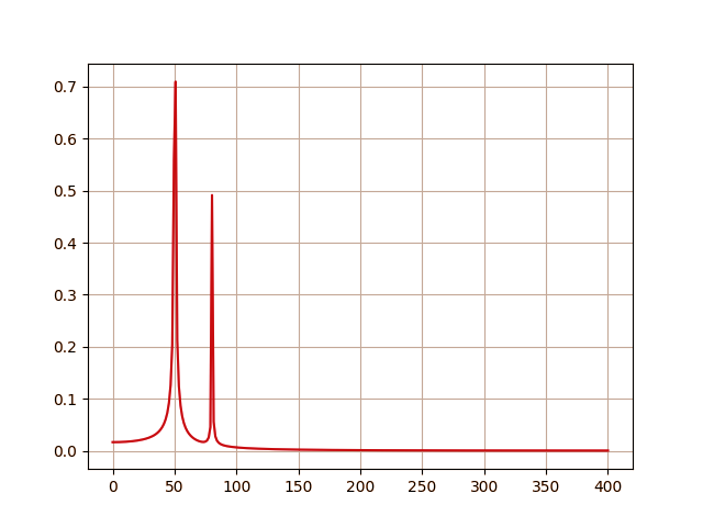
SciPy Tutorial – Fast Fourier Transforms

Special Functions of SciPy

The special module holds various transcendental functions that will help us with multiple tasks in mathematics.

To import it, use the following command-

>>> from scipy import special

We make use of the various functions:

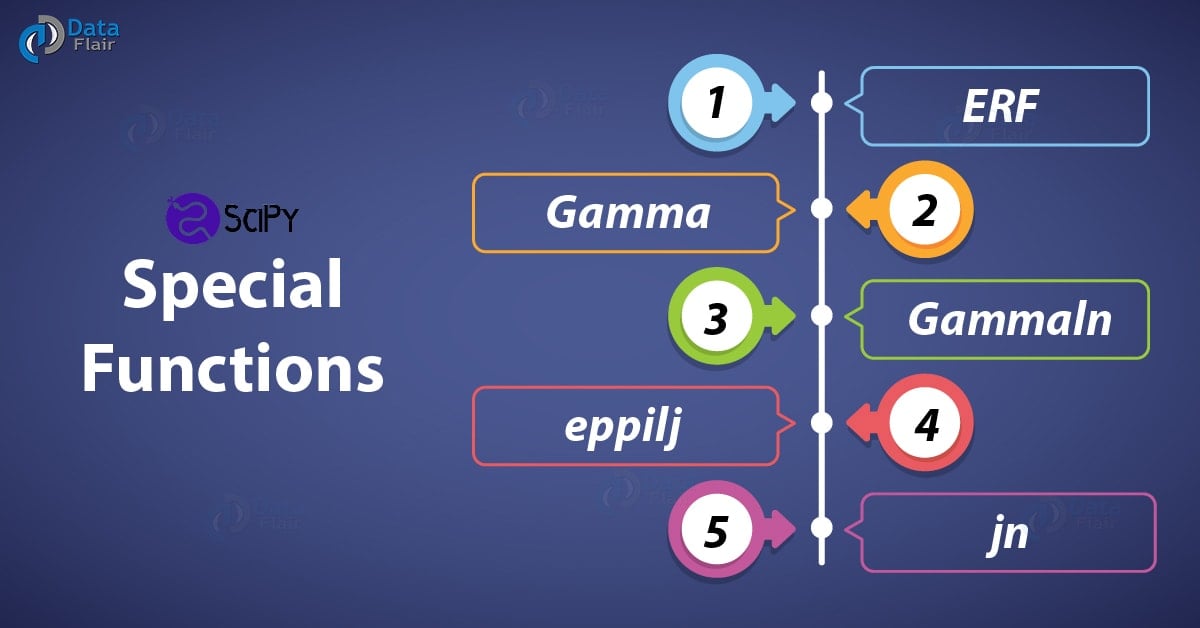
SciPy Tutorial – Special Functions of SciPy

1. ERF

This function calculates the area under a Gaussean curve. We use the erf() function.

2. Gamma

This calculates the Gamma. The function for this is gamma().

3. Gammaln

This calculates the log of Gamma. We use the function gammaln().

4. eppilj

The elliptic function we have is eppilj().

5. jn

This is the N^th order Bessel function.

Processing Signals with SciPy

SciPy will also help you with signal processing. Let’s take an example.

SciPy Tutorial – Processing Signals with SciPy

1. Using FFT to resample

We can resample a function to n points in a time domain interval. We can use the function resample() for this.

>>> t=numpy.linspace(-10,10,200)
>>> y=numpy.sin(t)
>>> from scipy import signal
>>> signal.resample(y,100)

Output

2. Removing Linear Trends

The detrend() function will remove the linear element from the signal; this gives us a transient solution.

>>> t=numpy.linspace(-10,10,200)
>>> y=numpy.sin(t)+t
>>> signal.detrend(y)

Output

Processing Images with SciPy

With SciPy, you can use ndimage to process images.

Some of the possible transitions are opening and closing images, geometrical transformation(shape, resolution, orientation), image filtering, and filters like erosion and dilation.

You can import it as:

>>> from scipy import ndimage

Let’s look at some functions we have:

1. Shift

This function will shift the image along the x and y coordinates. The function is shift(image,(x,y)).

2. Rotate

When you want to rotate your image to an angle, use the rotate(image, angle) function.

3. Zoom

With zoom(image, magnitude), you can zoom in or out on an image.

4. Median Filter

To filter an image with a Median filter, you can use median_filter(image, argument).

5. Gaussian Filter

And to filter with a Gaussian filter, you use gaussian_filter(image, argument).

6. Opening an Image in Binary

For this, you use the function binary_opening(image)

7. Closing an Image

To close this image, make a call to binary_closing(opened_image)

8. Binary Erosion

For this task, we use the function binary_erosion(image)

9. Binary Dilation

And to perform dilation, call binary_dilation(image)

Optimizing in SciPy

For algorithms that will optimize, we need the optimize package. Import it this way-

>>> from scipy import optimize

Let’s take a demo piece of code to explain this.

>>> from scipy.optimize import least_squares
>>> def func1(x):
             return numpy.array([10 * (x[1] - x[0]**2), (1 - x[0])])
>>> input=numpy.array([2, 2])
>>> res=least_squares(func1, input)
>>> res

Output

Working with Stats sub-packages of SciPy

The stats subpackage lets us work with statistics. Let’s take a few examples.
from scipy.stats import norm.

SciPy Tutorial – Working with Stats sub-packages of SciPy

1. CDF Removing Linear Trends

>>> norm.cdf(numpy.array([1,-1.,3,1,0,4,-6,2]))

This function computes the cumulative distribution at the points we mention.

2. PPF

For the Percent Point Function, we use the function ppf().

>>> norm.ppf(0.5)

Output

>>> norm.ppf(2.3)

Output

3. RVS

For a random variate sequence, use rvs().

>>> norm.rvs(size=7)

Output

4. Binomial Distribution

For this, we use the cdf() function from uniform.

>>> from scipy.stats import uniform
>>> uniform.cdf([0,1,2,3,4,5,6,7],loc=1,scale=3)

Output

So, this was all Python SciPy Tutorial. Hope you like our explanation.

Python Interview Questions on SciPy

1. What is SciPy in Python?
2. What is SciPy in Python used for?
3. How to import a SciPy module into Python?
4. What is SciPy optimize?
5. What is the difference between NumPy and SciPy in Python?

Conclusion

Hence, in this SciPy tutorial, we studied introduction to Scipy with all its benefits and Installation process.

At last, we discussed several operations used by Python SciPy like Integration, Vectorizing Functions, Fast Fourier Transforms, Special Functions, Processing Signals, Processing Images, Optimize package in SciPy.