ANOVA in R – A tutorial that will help you master its Ways of Implementation

In today’s era, more and more programmers are aspiring to become a Data Scientist. And, you must be aware that R programming is an essential ingredient for mastering Data Science. So, let’s jump to one of the most important topics of R; ANOVA model in R.

In this tutorial, we will understand the complete model of ANOVA in R. Also, we will discuss the One-way and Two-way ANOVA in R along with its syntax. After this, learn about the ANOVA table and Classical ANOVA in R.

Let’s start the tutorial.

What is ANOVA?

The ANOVA model which stands for Analysis of Variance is used to measure the statistical difference between the means. With the ANOVA model, we assess if the various groups share a common mean.  As a result, we have found that it’s used for investigating data by comparing the means of subsets of data.

Anova.glm

Generally, it’s an analysis of Deviance for Generalized Linear Model Fits.

As a result, it’s needed to compute an analysis of deviance table for one or more generalized linear model fits.

Learn everything about the Generalized Linear Models in R

Keywords:

models, regression

Usage:

# S3 method for glm
anova(object, …, dispersion = NULL, test = NULL)

Arguments:

1. the object, …

Basically, it’s the result of a call to glm or a list of objects for the “almost” method.

2. dispersion

Dispersion is defined as the parameter for the fitting family.

3. test

It’s a character string. As a result, it should match one of “Chisq”, “LRT”, “Rao”, “F” or “Cp”.

Implementing ANOVA in R

There are two ways of implementing ANOVA in R:

• One-way ANOVA
• Two-way ANOVA

One-way ANOVA in R

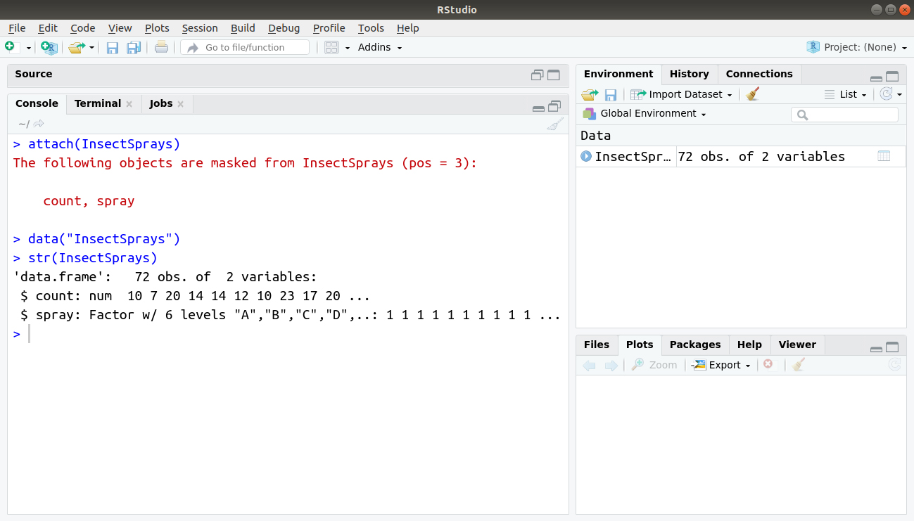
Let’s take an example of using insect sprays which is a type of data set. We are going to test 6 different insect sprays. As a result, we need to see if there was a difference in the number of insects found in the field after each spraying.

> attach(InsectSprays)
> data(InsectSprays)
> str(InsectSprays)

Output:

Do you know about Data Frame Operations in R

1. Descriptive Statistics

1. With the help of descriptive statistics, we calculate the mean, variance and number of elements in each cell.
   
2. Visualise the data – boxplot; look at the distribution for outliers.
   

We will be using tapply() here:

tapply() function is a very useful shortcut in processing data. Also, we use it as a function. It should be applied to each subset of the response variable defined by each level of the factor.

2. Run 1-way ANOVA

2.1 Oneway.test ( )

Use, for example:

> oneway.test(count~spray)

Output:

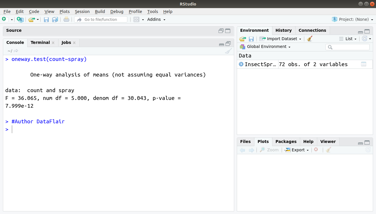
Default is equal variances not assumed that is Welch’s correction applied and this explains why the denom df (which is k*{n-1}) is not a whole number in the output O.

In order to alter this, we set the “var.equal =” option to TRUE.

Oneway.test( ) corrects the non-homogeneity but doesn’t give much information.

2.2 Run an ANOVA using aov( )

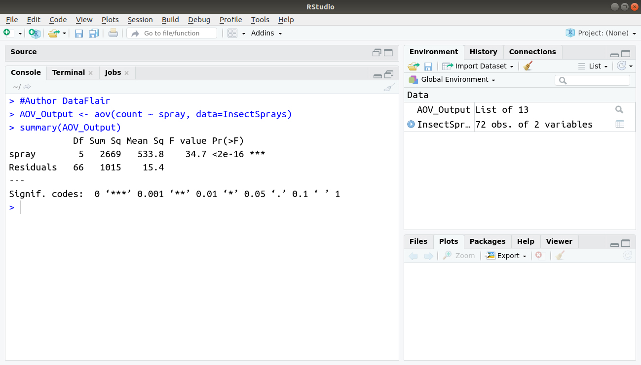
We use the aov() function to store the output and use extraction functions to obtain what is required.

> #Author DataFlair
> AOV_Output <- aov(count ~ spray, data=InsectSprays)
> summary(AOV_Output)

Output:

Have you checked – Survival Analysis in R

2. Two-way ANOVA in R

Two-way Analysis of Variance

We use it to compare the means of populations which is classified in two different ways. Besides, we can use lm() to fit two-way ANOVA models in R.

For example, the command:

> lm(Response ~ FactorA + FactorB)

fits a two- way ANOVA model without interactions. In contrast, the command:

> lm(Response ~ FactorA + FactorB + FactorA * FactorB )

includes an interaction term. Here, both FactorA and FactorB are categorical variables, while Response is quantitative.

Understand the complete concept of Factor Analysis in R

Classical ANOVA in R

Generally, we start with a simple additive fixed effects model. In this model, we use the built-in function aov:

aov(Y ~ A + B, data=d)

Now, to cross these factors or more for interacting with two variables, we use either of:

aov(Y ~ A * B, data=d)
aov(Y ~ A + B + A:B, data=d)

So far so good. Furthermore, we make an assumption that B is nested within A:

aov(Y ~ A/B, data=d)
aov(Y ~ A + B %in% A, data=d)
aov(Y ~ A + A:B, data=d)

Therefore, in nesting, we add both – the main effect and the interaction.

You must definitely explore the R Graphical Models tutorial

Random Effects in Classical ANOVA

aov can also deal with random effects that provides everything which is being balanced. Assume A is alone random effect, e.g. a subject indicator.

aov(Y ~ Error(A), data=d)

We make an assumption that A is random, B is fixed as well as nested within A. 

aov(Y ~ B + Error(A/B), data=d)

or B and X are crossed (interacted) within levels of random A.

aov(Y ~ (B*X) + Error(A/(B*X)), data=d)

Or B and X within random A are categorized by (non-nested) G and H:

aov(Y ~ (B*X*G*H) + Error(A/(B*X)) + (G*H), data=d)

As a result, this Error business can become confusing and the balance requirements, a bit tiresome. Thus, for random effects models, it’s usually easier to move to lme4.

Must Learn – Generalized Linear Models in R

ANOVA Table in R

Let’s say, we have collected data, and our X values have been entered in R as an array called data.X and Y values as data.Y.

Now, we will find the ANOVA values for the data. Then, follow the below steps:

• First, we will fit our data into a model. > data.lm = lm(data.Y~data.X).
• Next, we will get R to produce an ANOVA table by typing : > anova(data.lm).
• As a result, we will have an ANOVA table!

1. Fitted Values

Type:

> data.fit = fitted(data.lm)

to get the fitted values of the model.

As a result, it gives us an array called “data.fit” that contains the fitted values of data.lm.

2. Residuals

We use this to get the residuals of the model.

> data.res = resid(data.lm)

Now, as a result, we have an array of residuals.

3. Hypothesis Testing

• In case if we have already found the ANOVA table for our data, then we are able to calculate our test statistic from the numbers given.
• If we want to find the F – quantile given by F(.95;3,24)

Find this by typing:

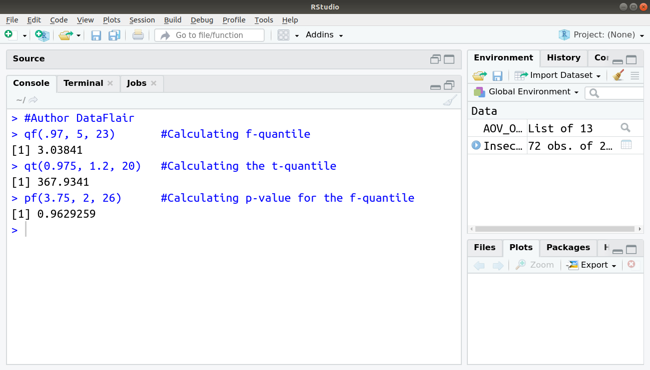
> #Author DataFlair
> qf(.97, 5, 23)

• If we want to find the t – quantile given by t(0.975, 1.2, 20)

Type:

> qt(0.975, 1.2, 20)       #Calculating the t-quantile

Output:

Don’t forget to check the Creation of Contingency Tables in R

4. P – values

In case if we want to get the p-value for the F – quantile of, say, 2.84, with degrees of freedom 3 and 24, we would type in

> pf(3.75, 2, 26)      #Calculating p-value for the f-quantile

5. Normal Q-Q plot

Generally, we use “data.lm to get the normal probability for the standard residuals of our data.

Although, we have already fit our data to a model, but now we will need the studentized residuals:

> data.stdres = rstandard(data.lm)

Also, type this to make the plot:

> qqnorm(data.stdres)

Then, to see the line, type:

> qqline(data.stdres)

Summary

We have studied ANOVA in R with their different types and properties. It is very much useful in investigating data by comparing the means of subsets of the data. Still, if you have any confusion regarding ANOVA in R, ask in the comment section.

For now, you must have a look at Chi-Square Test in R