Logistic Regression in R – A Detailed Guide for Beginners!
Job-ready Online Courses: Dive into Knowledge. Learn More!
In this tutorial, we will learn about the concept of logistic regression in R along with its syntax and parameters. We will also build a logistic regression model and explore its derivation, performance and applications.
Let’s quickly begin the tutorial.
What is Logistic Regression in R?
In logistic regression, we fit a regression curve, y = f(x) where y represents a categorical variable. This model is used to predict that y has given a set of predictors x. Hence, the predictors can be continuous, categorical or a mix of both.
It is a classification algorithm which comes under nonlinear regression. We use it to predict a binary outcome (1/ 0, Yes/ No, True/ False) given as a set of independent variables. Moreover, it helps to represent binary/categorical outcome by using dummy variables.
It is a regression model in which the response variable has categorical values such as True/False or 0/1. Therefore, we are able to measure the probability of the binary response.
Make sure that you have completed – R Nonlinear Regression Analysis
Syntax and Expression of R Logistic Regression
The general mathematical equation for logistic regression is:
y = 1/(1+e^-(a+b1x1+b2x2+b3x3+…))
Following is the description of the parameters used:
- y is the response variable.
- x is the predictor variable.
- a and b are the coefficients which are numeric constants.
We use the glm() function to create the regression model and also get its summary for analysis.
The syntax of logistic Regression in R:
The basic syntax for glm() function in logistic regression is:
glm(formula,data,family)
Description of the parameters used:
- Formula – Presenting the relationship between the variables.
- Data is the dataset giving the values of these variables.
- The family is the R object to specify the details of the model. Also, its value is binomial for logistic regression.
Derivation of Logistic Regression in R
We use a generalized model as a larger class of algorithms. Basically, this model was proposed by Nelder and Wedderburn in 1972.
The fundamental equation of generalized linear model is:
g(E(y)) = α + βx1 + γx2
Here, g() is the link function;
E(y) is the expectation of target variable, and
α + βx1 + γx2 is the linear predictor.
The role of the link function is to ‘link’ the expectation of y to linear predictor.
You must definitely check the Multiple Linear Regression in R
Performance of Logistic Regression Model
To test the performance of this model, we must consider a few metrics. Irrespective of a tool (SAS, R or Python) you would work on, always look for:
1. AIC (Akaike Information Criteria)
In logistic regression, AIC is the analogous metric of adjusted R². Thus, we always prefer the model with the smallest AIC value.
2. Null Deviance and Residual Deviance
- Null Deviance
In null deviance, the response that is predicted by the model is just an intercept.
- Residual Deviance
It indicates the response predicted by a model of adding independent variables.
3. Confusion Matrix
It is a type of matrix in which we represent a tabular representation of Actual vs Predicted values. Also, this helps us to find the accuracy of the model and avoid over-fitting.
Any queries in R Logistic Regression till now? Share your views in the comment section below.
Find out the best tool for Data Science Learning – R, Python or SAS
Building Logistic Regression Model in R
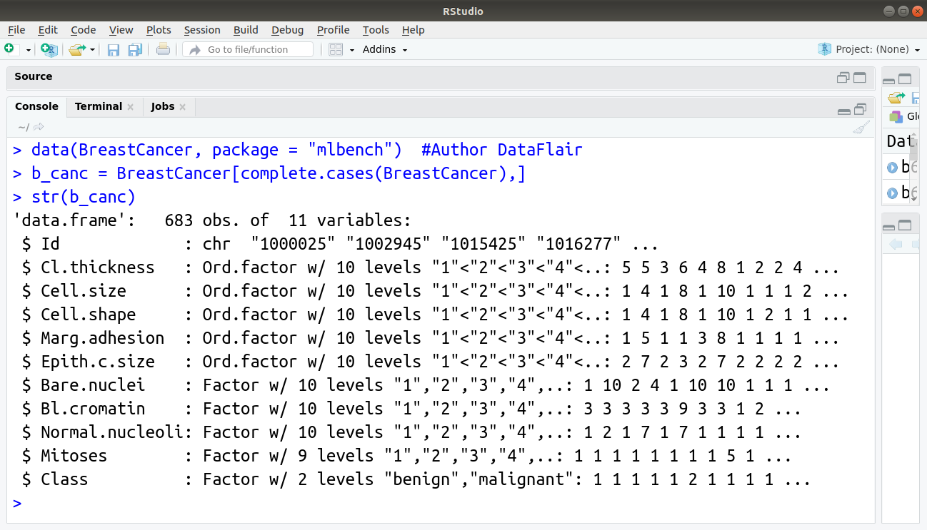
In this section, we will build our logistic regression model using the BreastCancer dataset that is available by default in R. We will start by importing the data and displaying the information related to it with the str() function:
> data(BreastCancer, package = "mlbench")  #Author DataFlair
> b_canc = BreastCancer[complete.cases(BreastCancer),]
> str(b_canc)
Output:
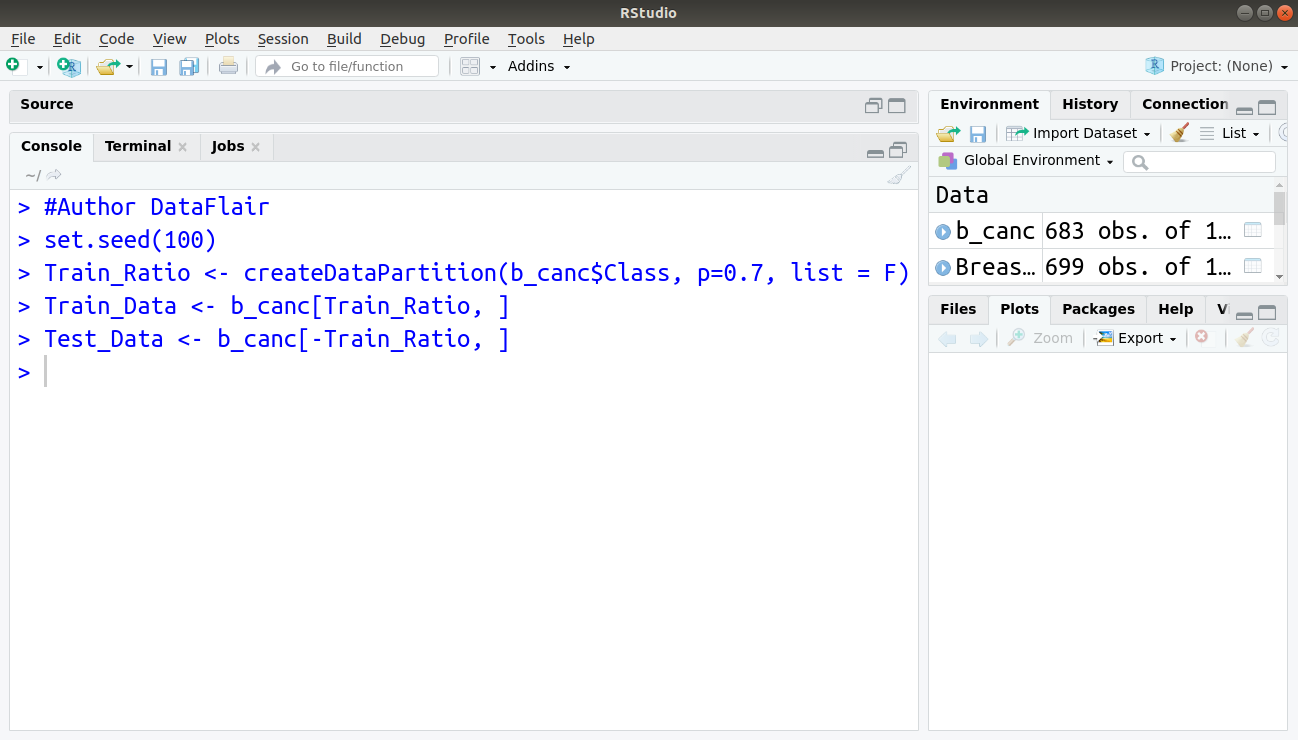
We now split our data into training and test set with the training set holding 70% of the data and test set comprising of the remaining percentage.
> #Author DataFlair
> set.seed(100)
> Train_Ratio <- createDataPartition(b_canc$Class, p=0.7, list = F)
> Train_Data <- b_canc[Train_Ratio, ]
> Test_Data <- b_canc[-Train_Ratio, ]
Output:
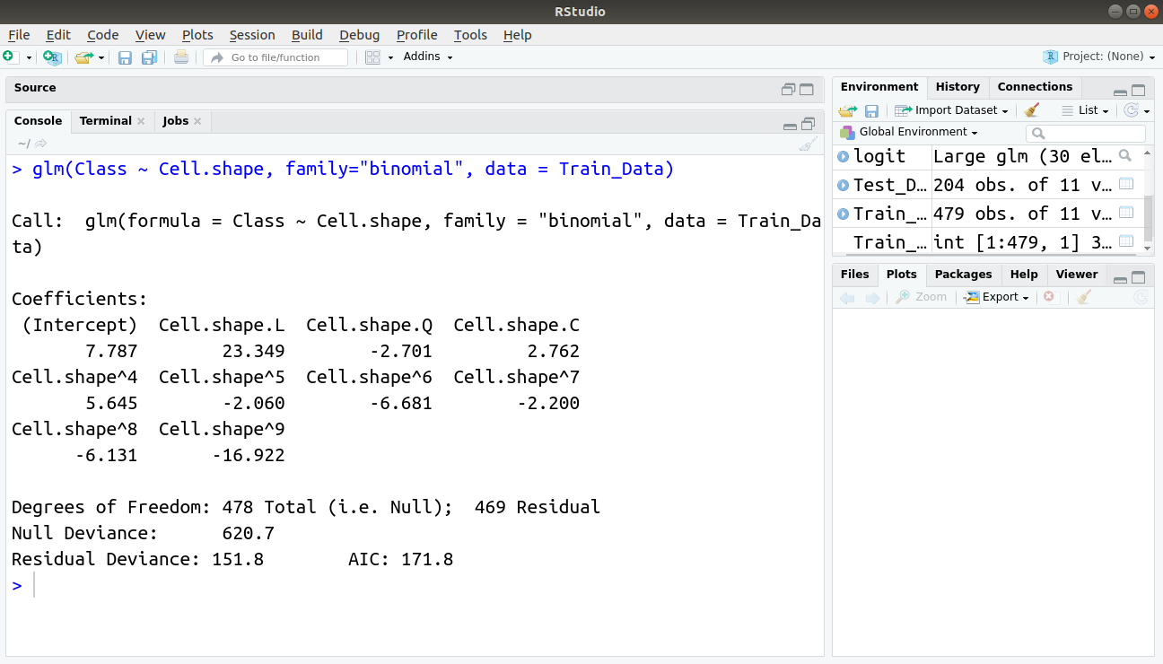
Implementing our logistic regression function using the function “lm” and specifying the attribute family as “binomial”, we obtain:
glm(Class ~ Cell.shape, family="binomial", data = Train_Data)
Output:
Applications of Logistic Regression with R
- It helps in image segmentation and categorisation.
- Generally, we use logistic regression in geographic image processing.
- It helps in handwriting recognition.
- We use logistic regression in healthcare. That is an application area of logistic regression.
- To make predictions about something that we use in logistic regression.
Summary
As a result, we have seen that logistic regression in R plays a very important role in R Programming. Therefore, with the help of this algorithm, we can conclude the important binary results. As we have discussed its syntax, parameters, derivations as well as examples. Also, we looked at the Logistic Regression Model in R with its performance.
Now, it’s time to Create Decision Trees in R Programming
Still, if you feel any confusion regarding R Logistic Regression, ask in the comment tab.
Did we exceed your expectations?
If Yes, share your valuable feedback on Google


