R Programming Interview Questions for aspiring Data Scientists [Updated]

Welcome back to R Programming Interview Questions and Answers Part 2.

DataFlair has published a series of R programming interview questions and answers that will help both beginners and experienced of R and data science to crack their upcoming data scientists interview. Bookmark the links and practice the questions –

• R Language Interview Questions and Answers for Freshers
• R Language Interview Questions and Answers for Intermediate Level
• R Language Interview Questions and Answers for Experienced

Let’s continue to the second part – R programming interview questions and answers for data scientists. This part mainly focuses on R coding interview questions and technical interview questions. Now, you will not face any difficulty in your tech round. Do practice all the questions and get ready for the upcoming interviews.

In between, if you feel you need to revise any concept you are not clear with you can comment below or check the Free R Tutorials Library

R Coding Interview Questions and Answers

Q.1 What is f(3) where:

x <- 7
f <- function(y) { x <- 3; x^2 + g(y) }
g <- function(y) { y + x }

Ans. The above-written code will return the result of 19. In f In f(3), x is 3, so x^2 is 6. Then, the value is passed to g(3), where x is globally scoped and hence y + x = 3 + 7 = 10. Hence, we obtain f(3) = 9 + 10 = 19 as the final answer.

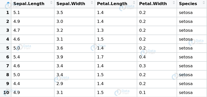
Q.2 Given the IRIS dataset, consisting of a mix of continuous variables and categorical ones.

Where would you apply –

• Barplot
• Histogram

Also, explain where do these two types of plots differ with their respective implementations.

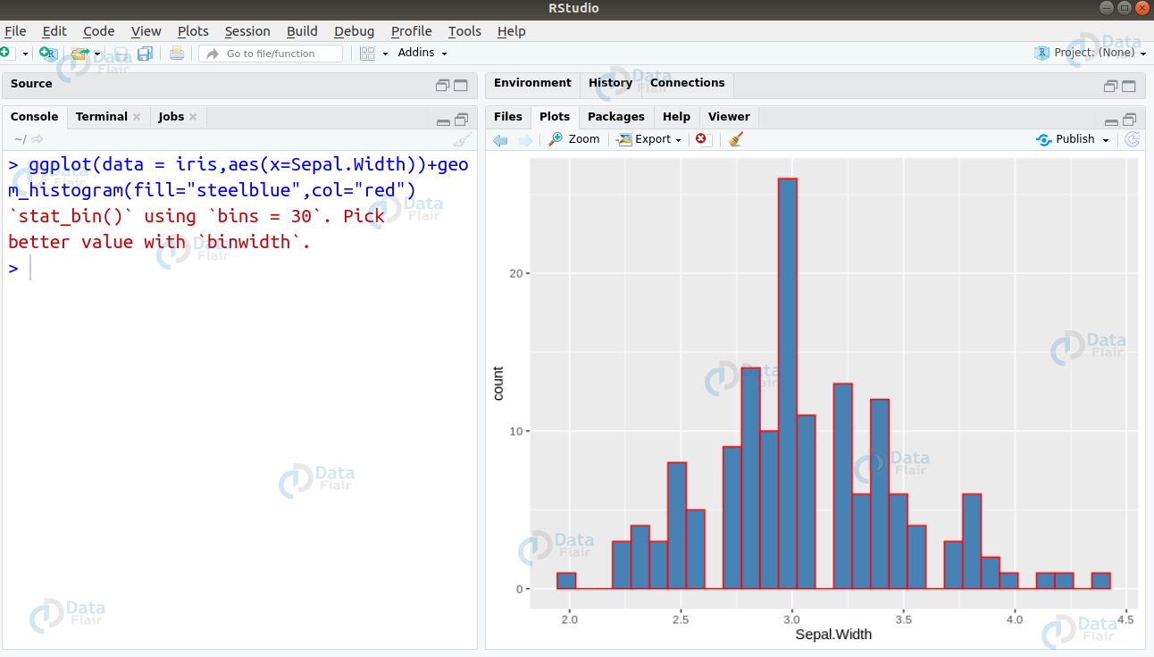
Ans. Histograms are used for plotting continuous variables. On the contrary, Barplots are used for plotting categorical variables. In the given data, Species column consists of categorical data whereas rest of the data consists of continuous one. We can plot a histogram for the feature Sepal.Width as follows –

> ggplot(data = iris,aes(x=Sepal.Width))+geom_histogram(fill="steelblue",col="red")

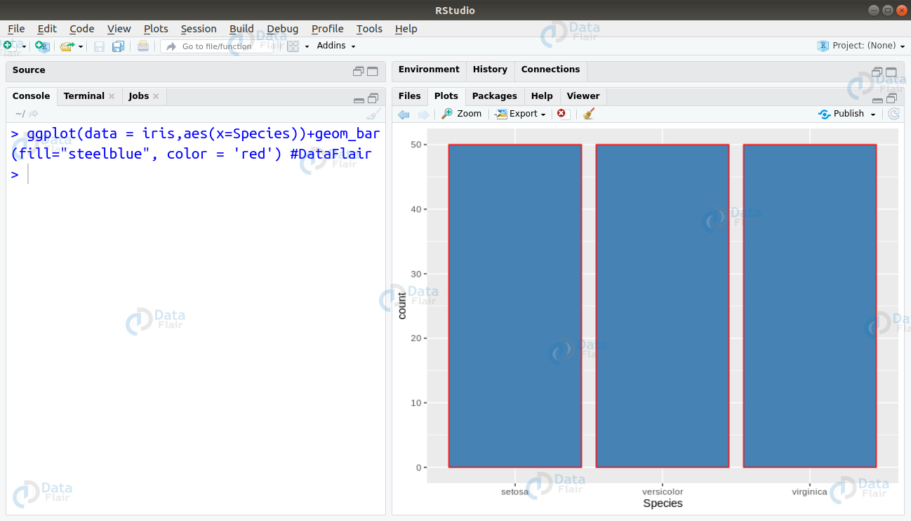
Furthermore, for plotting a barplot, we write the following line of code –

> ggplot(data = iris,aes(x=Species))+geom_bar(fill="steelblue",color = 'red') #DataFlair

Learn in detail about Barplot and Histogram

Q.3 Suppose you have to work on a dataset consisting of categorical variables. Let this dataset be iris which consists of the column “Species” being categorical in nature. You have to implement the XGBoost Algorithm. What problem would you face and how will you resolve it?

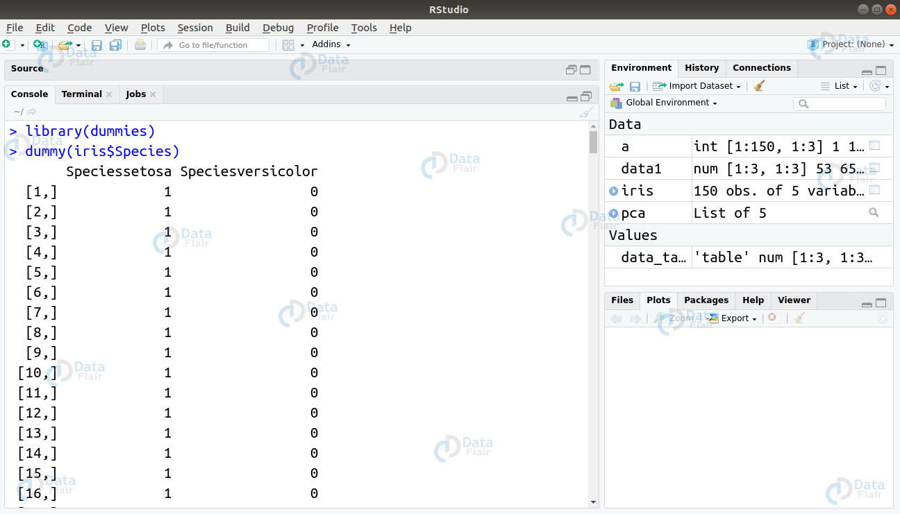
Ans. The XGBoost Algorithm only works well with the numerical data. Considering that we have a categorical feature – “Species” in our dataset, we will first have to convert that into numerical form. This can be achieved by using dummy variables. We can implement this as follows –

library(dummies)
dummy(iris$Species)

Q.4 In the same iris dataset, you have been assigned the task of identifying outliers. You must be able to provide a comprehensive glimpse of the dataset using a suitable visualisation. What method would you choose and why?

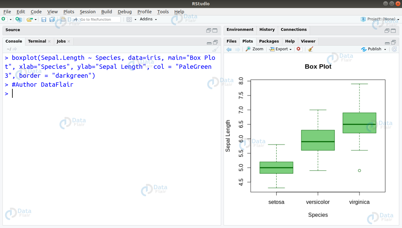
Ans. Visualising Boxplot is an ideal method of identifying the outliers. The identification of outliers is important because through boxplots, one can obtain a comprehensive idea of the minimum, lower quartile (25th percentile), median (50th percentile), upper quartile (75th percentile), as well as the maximum of a continuous variable. This will help us to get an overall idea of how the data is, and if there are any outliers which may affect the fitting of our model.

Here is a detailed guide for Data Visualization with R

We can create our boxplot on the iris dataset as follows –

boxplot(Sepal.Length ~ Species, data=iris, main="Box Plot", xlab="Species", ylab="Sepal Length", col = "PaleGreen3", border = "darkgreen")

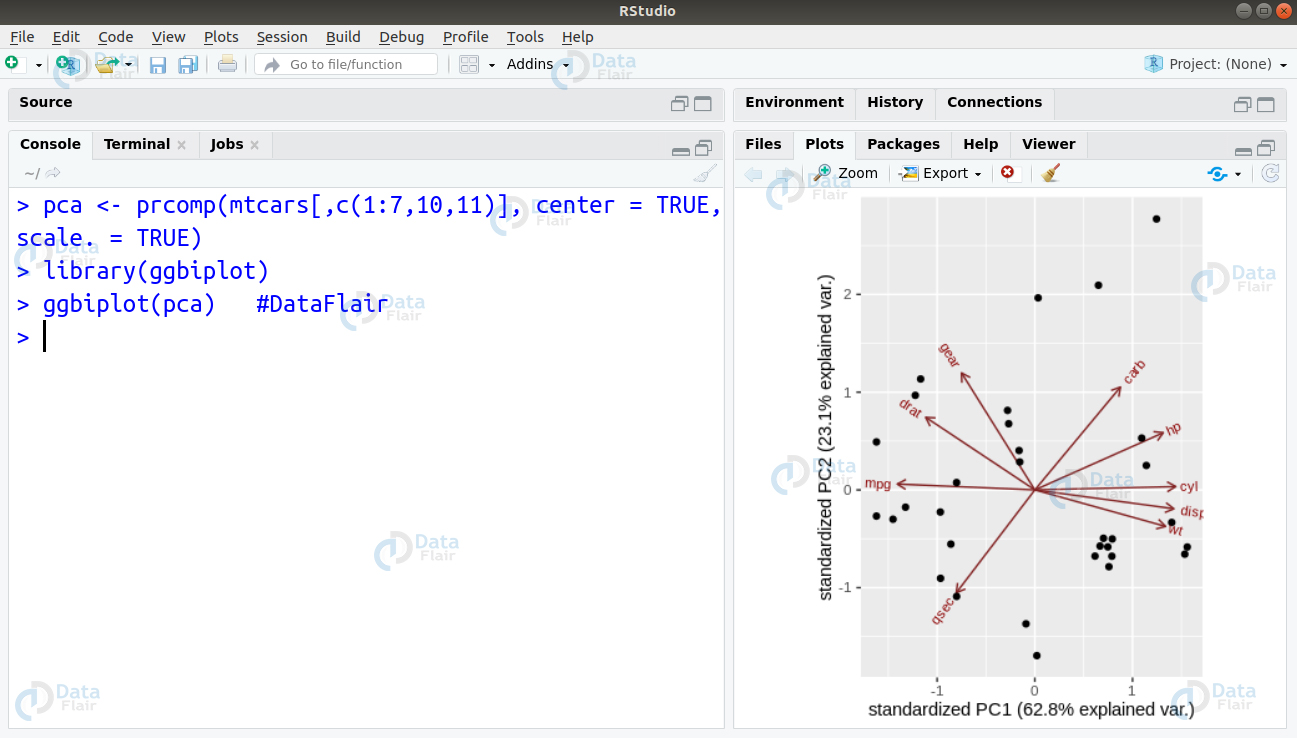
Q.5 Given a dataset, you wish to explore the variations that are present in the features. However, suppose that the dataset consists of 1000 features. It is not easy to represent all of these features in a single plot to gain an idea of the trends contained within. What will you do in this scenario? For simplicity of implementation, consider the mtcars dataset present in the R environment.

Ans. This problem statement requires us to implement Principle Component Analysis. With the help of this algorithm, one can easily see the overall shape of the data. Through visualisation of the variations in the data, one can identify similar features as well as dissimilar features. In order to implement PCA on this dataset, we must first drop the ‘vs’ and ‘am’ variable as they are categorical in nature. We will then plot our PCA graph with rest of the dataset –

> pca <- prcomp(mtcars[,c(1:7,10,11)], center = TRUE,scale. = TRUE)
> library(ggbiplot)
> ggbiplot(pca) #DataFlair

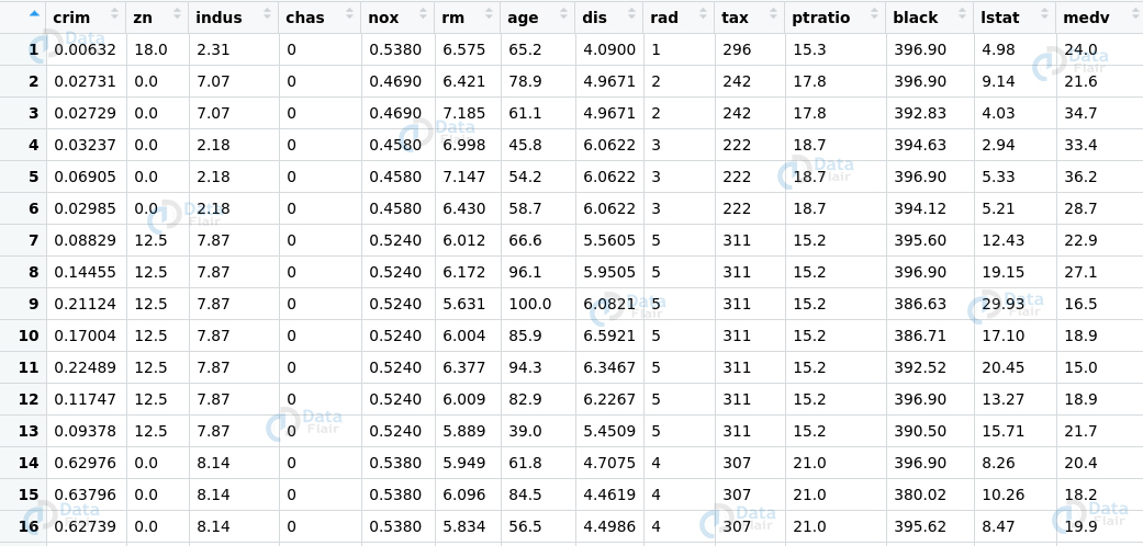
Q6. How do correlated variables in a dataset affect the model performance? Given the ‘boston’ dataset provided by R, diagnose the model to improve its performance.

Ans. While carrying out regression, it is assumed that the variables are not correlated to one another. If the variables are however, correlated then our model will suffer from the following problems.

• The parameters present in our model will become indeterminate.
• During model evaluation, the standard error of the estimated values will increase significantly.

Furthermore, the solution of our regression model will become highly unstable. In order to compute multicollinearity present in our dataset, we make use of the Variance Inflation Score or VIF. This score measures the inflation caused to the correlation coefficient contributed by multicollinearity that is present in the model.

To check for multicollinearity in our model. We will begin by splitting the boston dataset into training and test data.

> set.seed(123)
> sample_data <- Boston$medv %>%
+ createDataPartition(p = 0.8, list = FALSE)
> training_data <- Boston[sample_data, ]
> testing_data <- Boston[-sample_data, ]
> #DataFlair

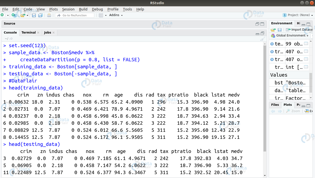
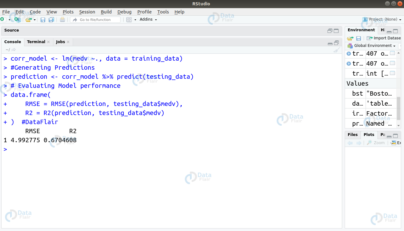
In the next step, we will build a regression model and evaluate its accuracy.

Now, we will evaluate the VIF score for each variable

car::vif(corr_model)

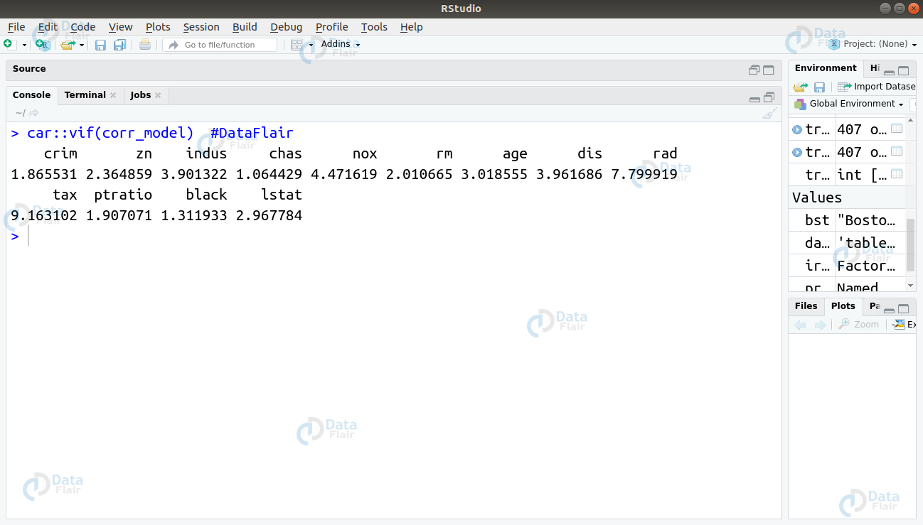
From the VIF scores generated above, we observe that the tax variable has the highest score. Therefore, we will remove this variable and evaluate our model again.

> # Building the model without tax variable #DataFlair
> corr_model <- lm(medv ~. -tax, data = training_data)
> # Generate Predictions
> prediction <- corr_model %>% predict(testing_data)
> # Model performance
> data.frame(
+    RMSE = RMSE(prediction, testing_data$medv),
+    R2 = R2(prediction, testing_data$medv)
+ )

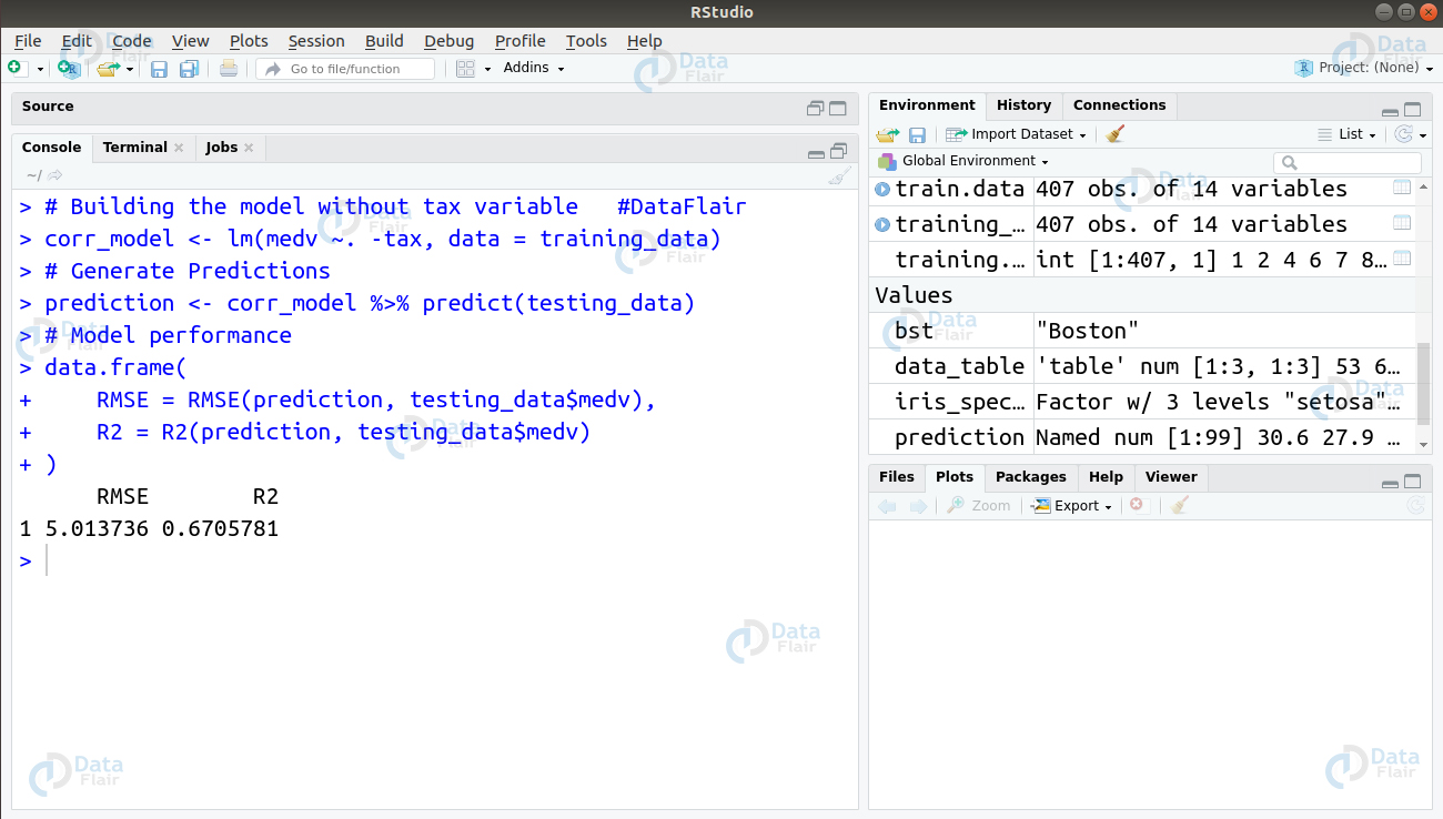
From the above observation, we conclude that removing ‘tax’ variable does not affect the model much. Therefore, the model requires other areas of improvement to achieve a better score.

Q.7 What will be the output of this code? State the reason behind the flow of code execution.

generic2 <- function(x) UseMethod("generic1")
generic2_a1 <- function(x) "a1"
generic2_a2 <- function(x) "a2"
generic2_b1 <- function(x) {
  class(x) <- "a1"
  NextMethod()
}


generic2(structure(list(), class = c("b1", "a2")))

Ans. After we run the above code, following things happen in the code –

• The objects of class b1 and a2 get passed to generic(). This prompts the R code to search for the method we pass an object of class b and a2 to generic2(), which prompts R to look for a method generic2_b1()
• The generic2_b1() method changes class the class to a1 and then the NextMethod().
• Normally, one would assume that R will call genericOne would think that this will lead R to call generic2_a1(). However, the NextMethod() does not work with the class attribute but instead makes use of the global variable (.Class) that monitors next method to be called.

Therefore, in the above code, generic2_a2() is called.

Q.8 Will the following code return any error? State the reason behind your answer.

val <- numeric()
result <- vector("list", length(val))
for (index in 1:length(val)) {
  result[index] <- val[index] ^ 2
}
result

Ans. The code will not yield any error. In the above code, the index iterates over the vector val having a length of 0. The loop is taken from index = 1 to index = 0. The ‘:’ in this case counts down. During the first iteration, val[1] will have an NA indexing for the atomic value. This resulting NA will have an empty length give the result[1] – “out of bounds indexing for the lists”

In the following iteration, val[0] will provide us with the numeric(0) index as a returned value. Squaring the value will not have any effect and as a result, numeric(0) is assigned to result[0]. When a vector of length 0 is assigned to a subset of length 0, it does not alter anything. The code will execute as it step involves valid R operations.

Q.9 Import the diamonds dataset that is provided by the ggplot package. Your aim is to create a scatter plot of price vs depth. How will you proceed to find the depth value where most diamonds are found?

Ans. Using ggplot2 package, we will plot the scatterplot of the variable depth vs price as follows –

ggplot(data = diamonds, aes(x = depth,y = price)) +
+ geom_point(alpha= 0.5) #DataFlair

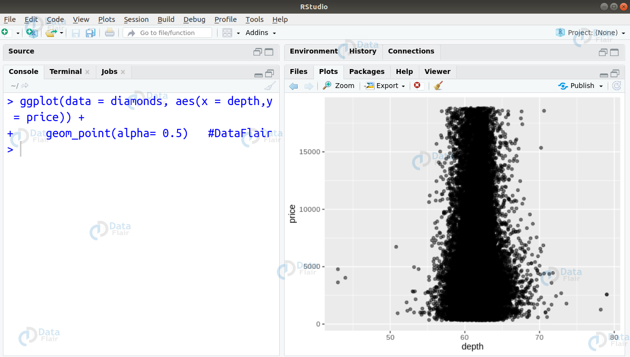
We can observe that the diamonds are densely concentrated in an area around 60. However, this does not give us a precise area where the highest concentration of diamonds of located. Therefore, we change the transparency of the points to be 1/100th of their original and mark the x-axis at every 2 units.

ggplot(data = diamonds, aes(x = depth,y = price)) +
+ geom_point(alpha= 0.01) +
+ scale_x_continuous(breaks = seq(0,80,2))

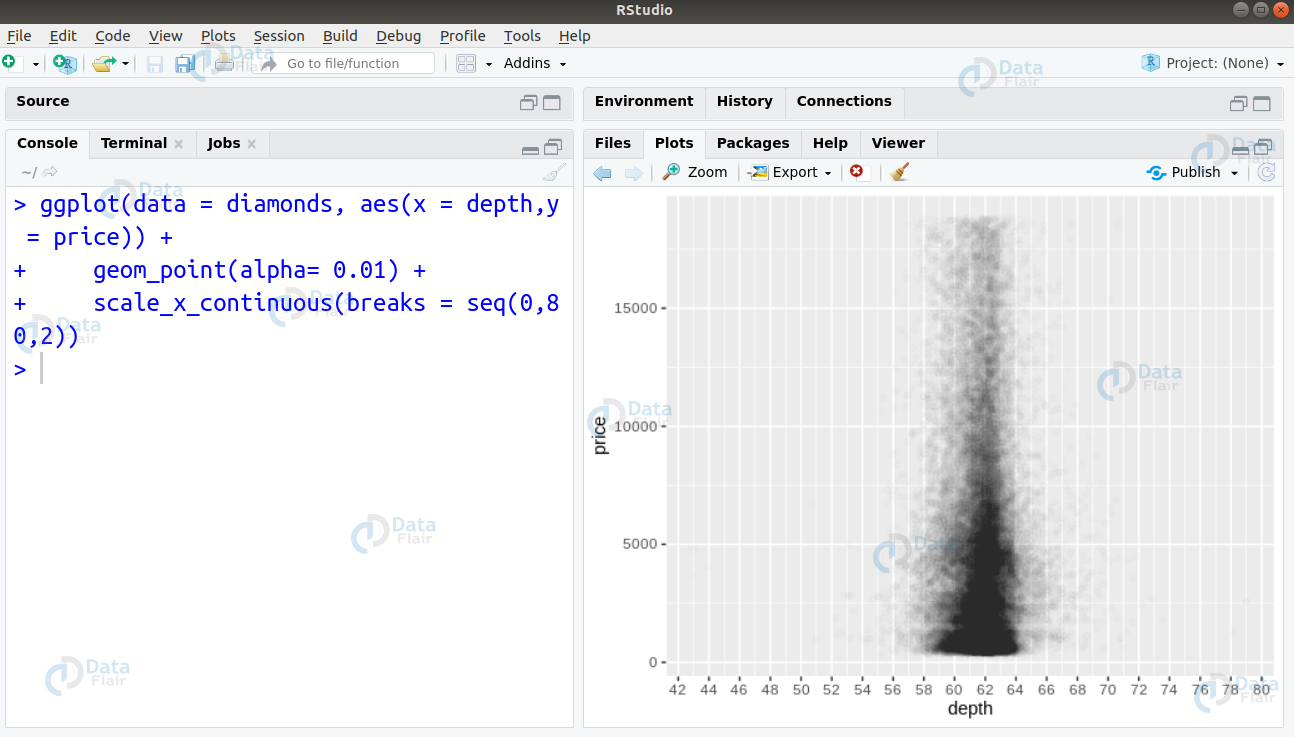
From the above visualisation, we observe that the highest concentration of diamonds is between 60-64.

Don’t miss to revise the important concept of R packages for your upcoming data science interviews

Q.10 What are some of the errors present in the code below? Fix these errors with their respective correct answers.

• iris[iris$Sepal.Length = 5, ]
• iris[-1:5, ]
• iris[iris$Sepal.Length <= 5]

Ans. The correct versions of these codes are as follows –

• iris[iris$Sepal.Length == 5, ]
• iris[-(1:5), ]
• iris[iris$Sepal.Length <= 5, ]

Q.11 Suppose that you want to access a graphics device, run the code on it and then close the device. How will you carry out this procedure in the form of a function? The file that you want to save is a pdf file – ‘data.pdf’

PDF_plot <- function(code) {
  pdf("data.pdf")
  on.exit(dev.off(), add = TRUE)
  code
}

Q.12 How will you convert the following code into its corresponding prefix form?

2 + 3 + 4
2 + (3 + 4)
if (length(x) <= 5) x[[5]] else x[[n]]

Ans. Let us rewrite these expressions to match the given code syntax. Since the prefix functions pre-define the order of execution, the parentheses can be therefore, omitted in the second expression.

`+`(`+`(2, 3), 4)

`+`(2, `(`(`+`(3, 4)))
`+`(2, `+`(3, 4))

Important Tip!! If you want to crack your next data science interview so along with these top R programming Interview Questions and Answers you need to practice some R projects.

DataFlair has published many projects, practice here – Top R projects for Data Science interview

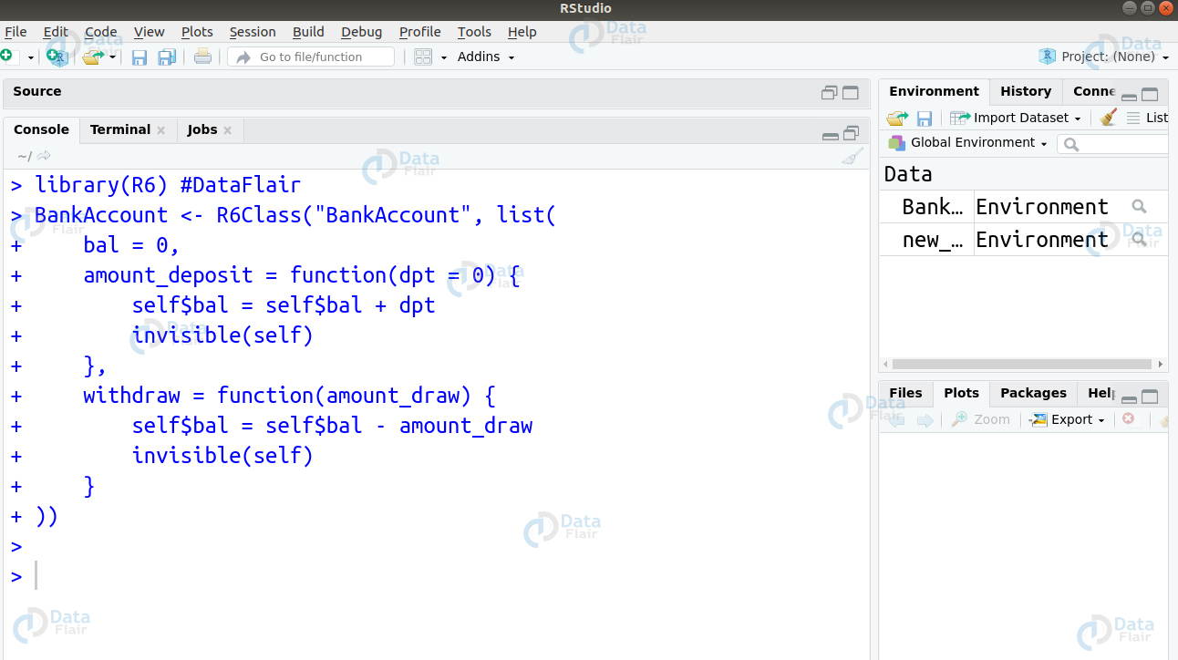
Q.13 How will you create an R6 class that lets you have a bank account you to access your balance, store deposit as well as withdraw money?

Ans.

BankAccount <- R6Class("BankAccount", list(
bal = 0,
amount_deposit = function(dpt = 0) {
  self$bal = self$bal + dpt
  invisible(self)
},
withdraw = function(amount_draw) {
  self$bal = self$bal - amount_draw
  invisible(self)
}
))

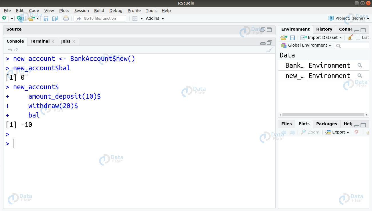
Let us test this by creating an instance and getting a balance.

new_account <- BankAccount$new()
new_account$bal
new_account$
 amount_deposit(10)$
 withdraw(20)$
  bal

Q.14 How will you create an R6 class that manages the current working directory? This class should have $get and $set() methods.

Ans. The R6 class for managing the current working directory be implemented as follows –

WorkingDirectory <- R6Class("WorkingDirectory", list(
  get_directory = function() {
    getwd()
},
set_directory = function(value) {
    setwd(value)
}
))

Q.15 What takes place when you alter the levels of a factor given below?

fac <- factor(letters)
levels(fac) <- rev(levels(fac))

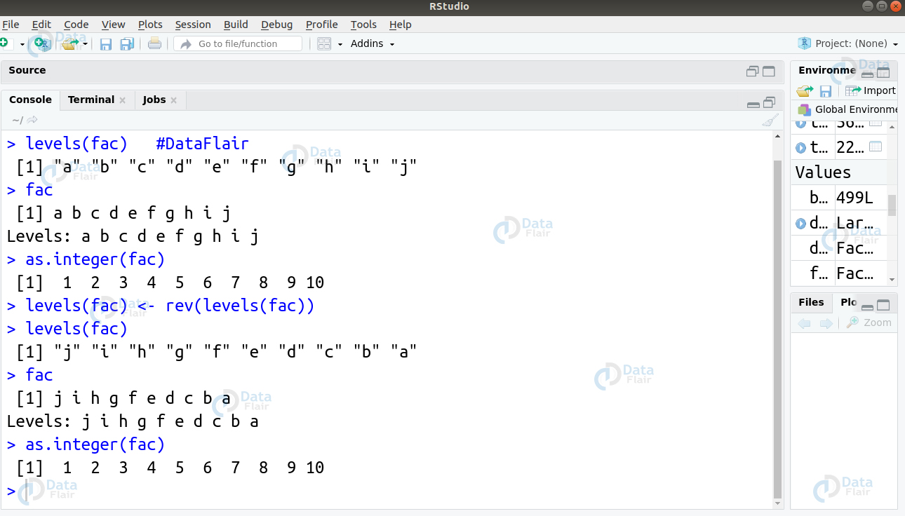
Ans. The various integer values that lie in the factor remain the same. However, the levels get altered giving the data a changed appearance.

> fac <- factor(letters[1:10])
> levels(fac) #DataFlair
> fac
> as.integer(fac)
> levels(fac) <- rev(levels(fac))
> levels(fac)
> fac
> as.integer(fac)

Q16. Suppose you have a character vector containing the strings as follows –

(string1 <- c("a", "ab", "adb", "addb", "adddb", "adddb"))

You want to utilize a regex operation that would match the strings for the different variations in the pattern ‘adb’. You have to perform pattern matching in two ways –

• For atleast 1 time
• For atleast 0 time

How will you carry out this operation?

Ans. In order to obtain the two outputs, we will make use of the grep() function. This function takes the regex as first argument and input vector as its second argument. In this case, we will pass value = TRUE as we want the grep to return the vector being a copy of the actual elements in the input vector that can be matched. The two regex operations we will utilize for obtaining the desired output are –

• ad*b
• ad+b

These two operations differ in their quantifier that defines how many times an object must be repeated. The ‘*’ quantifier would match the repetition atleast 0 times and the ‘+’ quantifier would perform it atleast 1 time. Then, we will implement this in code as follows –

grep("ad*b", string1, value = TRUE)

grep("ad+b", string1, value = TRUE)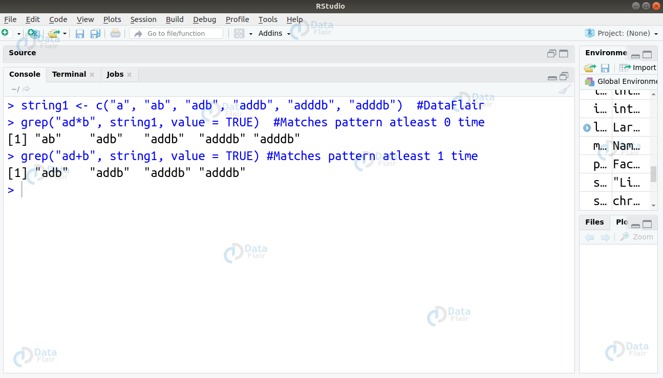

R Functions – A very helpful article for R programming interview questions 

Q.17 You have a task of finding names of all the .csv files in the repository. How will you carry this out using the regex operation? These csv files are stored in the following pattern –

[1] “birds.csv” “boston.csv” “data.csv” “grass.csv” “table.csv”

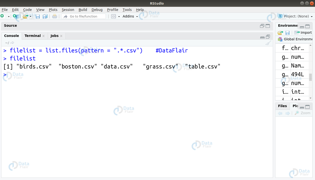
Ans. In this, we will make use of the combination of two regex quantifiers – ‘.’ and ‘*’. The ‘.’ quantifier returns the match found in any single character. We will create a character variable ‘csvlist’ and use the list.files() function with the pattern = “.*.csv” as follows –

csvlist = list.files(pattern = ".*.csv")

Q.18 Suppose that you have string as follows –

data_string <- “I learn Big Data for 4 hours daily with DataFlair”

You have to perform following operations using various regex sequences –

• Match the digit 4 and replace it with a dash ‘_’
• Replace the non-digit part of the string with ‘_’
• Replace the non-word character in string with ‘&

Ans.

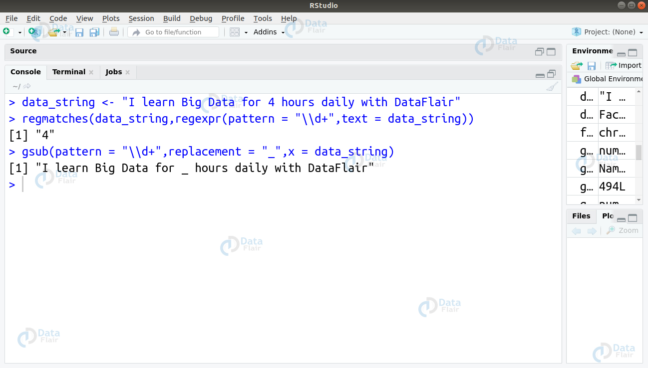
1. For matching the digit and replacing it with ‘_’, we will make use of the gsub() and regmatch() function as follows –

gsub(pattern = "\\d+",replacement = "_",x = data_string) 
regmatches(data_string,regexpr(pattern = "\\d+",text = data_string))

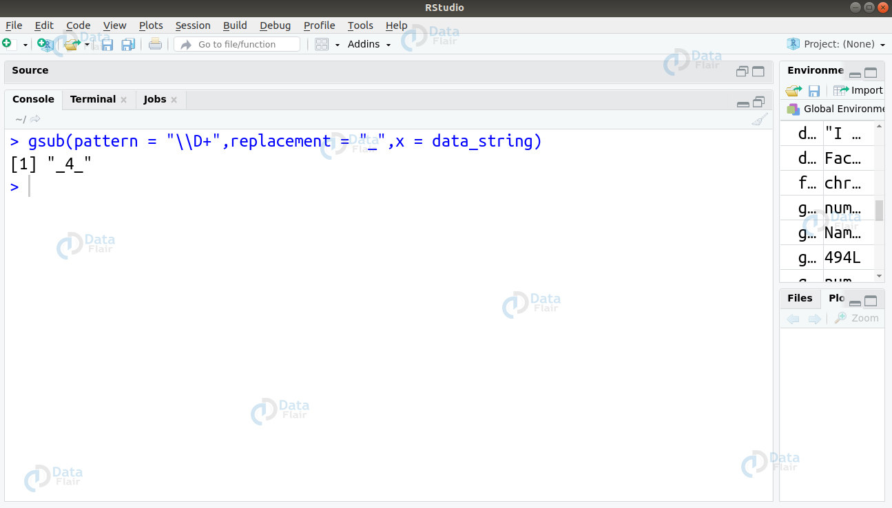
2. To match the non-digit part of the string and replace it with ‘_’, we will use the \D sequence to match the non-digit part of our string and replace it with ‘_’.

gsub(pattern = "\\D+",replacement = "_",x = data_string)

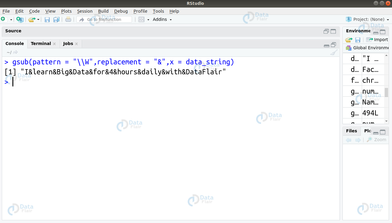
3. To match the non-word character and replace it with ‘&’, we will use the sequence \W as follows –

> gsub(pattern = "\\W",replacement = "&",x = data_string)

Q.19 For a given string, you have to extract all the email addresses that are contained in it.

email <- c("My email is [email protected]","my email address is [email protected]","John Wayne","Clint Eastwood")

Ans. To carry out this operation, we will make use of the POSIX class. In particular, we will use the [[:alnum:]] and [[:alpha:]] classes. The alnum class matches the alphanumeric characters whereas alpha class matches the letters.

> email <- c("My email is [email protected]","my email address is [email protected]","John Wayne","Clint Eastwood")
> unlist(regmatches(x = email, gregexpr(pattern = "[[:alnum:]]+\\@[[:alpha:]]+\\.com",text = email)))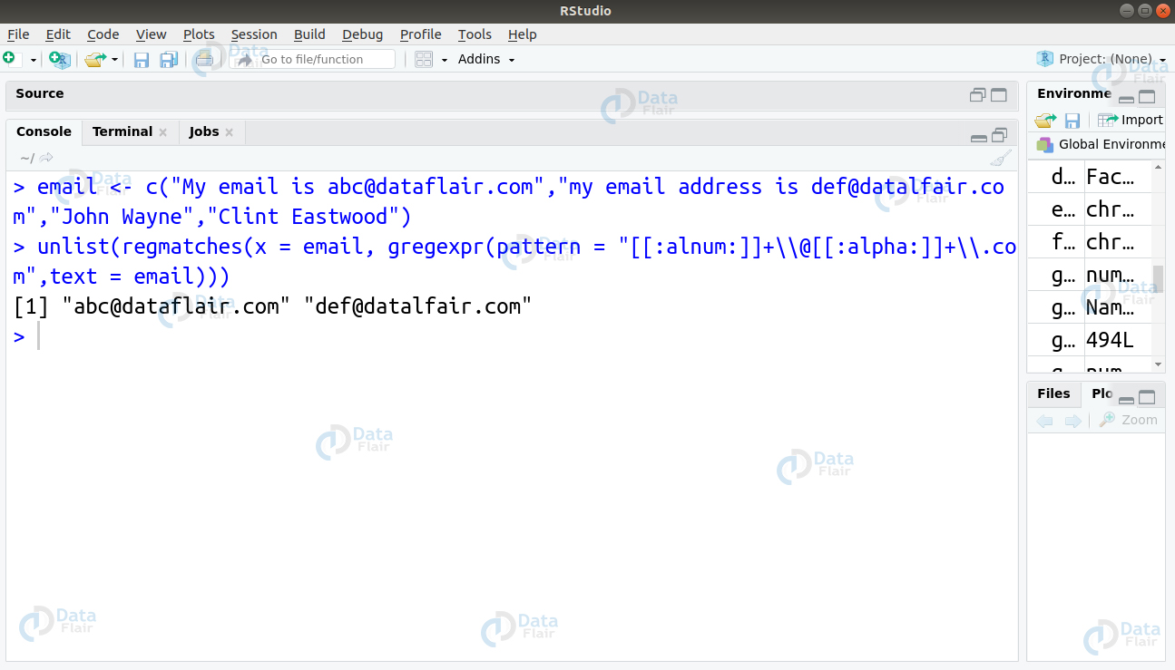

Q.20 Suppose you have to deal with a dataset. In this case, we will use the USArrests dataset provided by R.

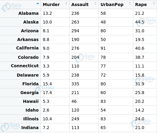
Before you proceed ahead with the model implementation. You have to perform data transformation in the following ways –

• Abbreviate the names of states.
• Select the states that contain the letter ‘b’
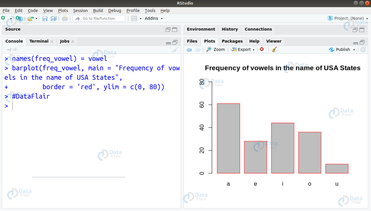
• Count the frequency of the vowels in and plot their frequency distribution plot.

Ans.
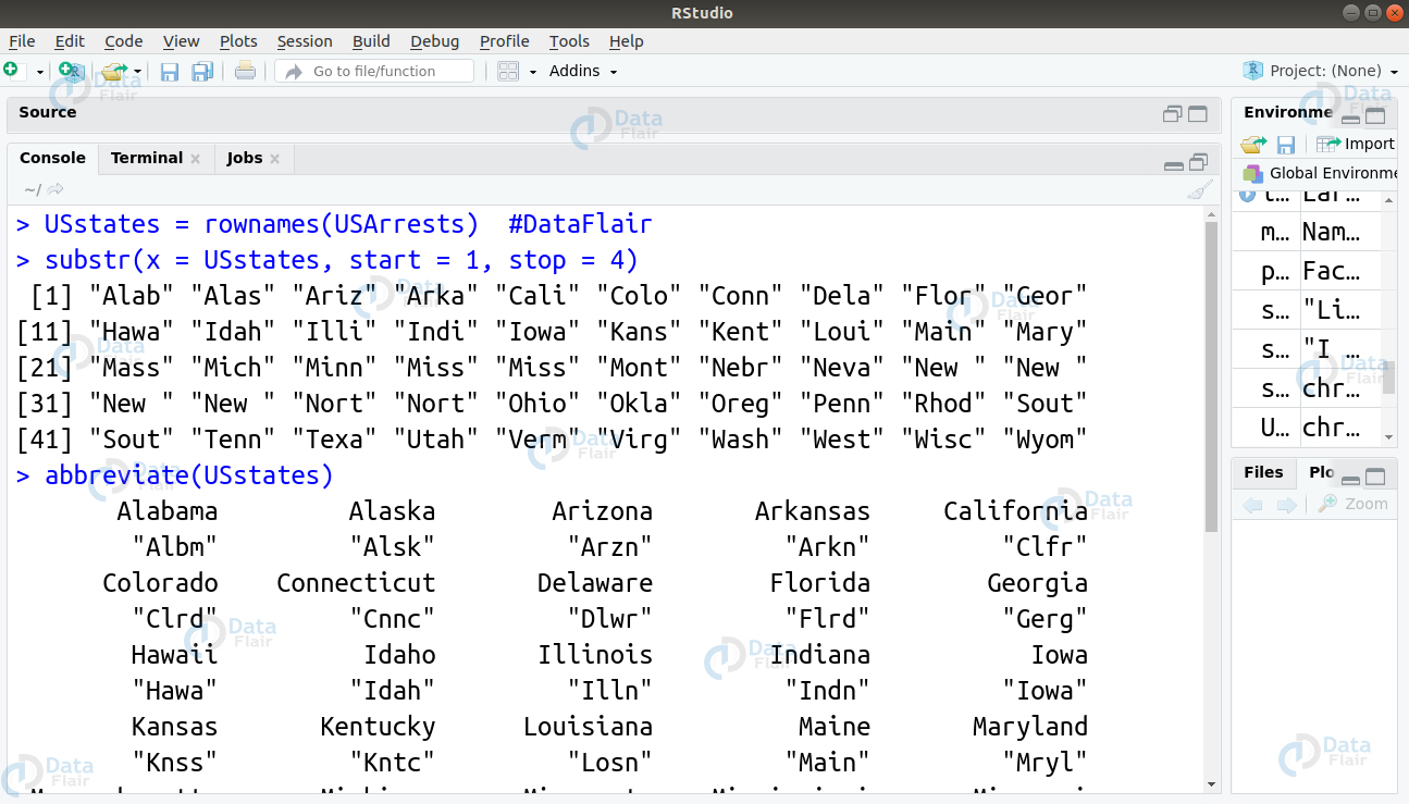
There are two ways to abbreviate names of the states –

• Firstly, we can use the substr() function to limit the names of our states to a length of 4.

substr(x = USstates, start = 1, stop = 4)

• Secondly, we can use the abbreviate() function as follows –

abbreviate(USstates)

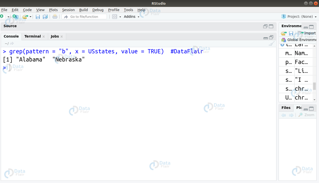
To select the states containing letter “b”, we will use the grep function as follows –

grep(pattern = "b", x = USstates, value = TRUE)

To count the frequency of vowels, we will write the following code:

vowel = c("a", "e", "i", "o", "u")
freq_vowel = vector(mode = "integer", length = 5)
for (index in seq_along(vowel)) {
    num_total = str_count(tolower(states), vowel[index])
    [index] = sum(num_total)
}
names(freq_vowel) = vowel #DataFlair
freq_vowel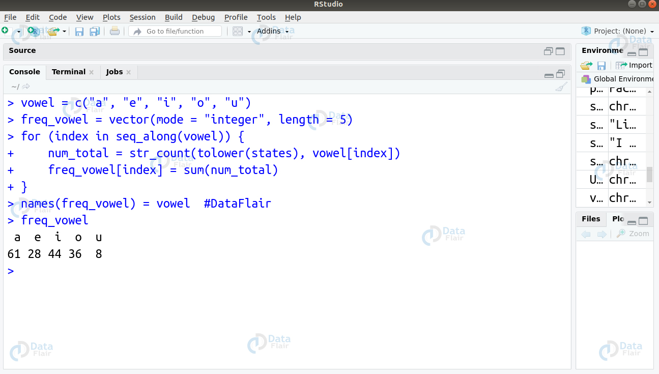

Then, we will plot a histogram to count the frequency of vowels occurring in the states.

barplot(num_vowels, main = "Number of vowels in USA States names", border = NA, ylim = c(0, 80))

This type of R programming question is mostly asked for interview. Practice more such questions.

Q 21. What conditions hold true in a stationary time-series analysis? Given the dataset ‘EuStockMarkets‘, how will you impose these conditions on it?

Ans. If the following conditions hold true, then the time-series model is said to be stationary –

• The average value of the time-series model is constant with the passage of time. Therefore, the trend component will be void.
• The model variance does not increment over time.
• The effect of seasonality is negligible.

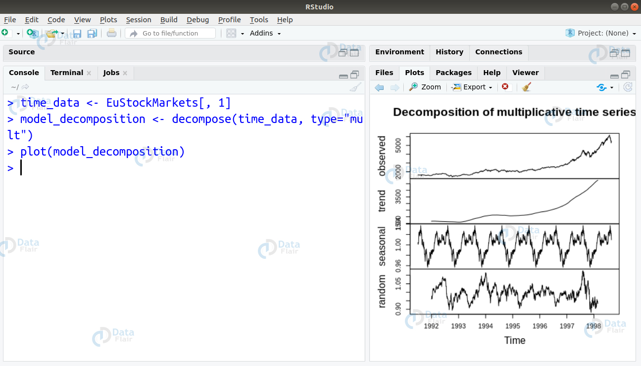
Therefore, a stationary time-series model does not have a trend or seasonal pattern making it look similar to the white noise. This is irrespective of the observed time intervals. We can impose these conditions by extracting the trends, seasonality and errors as follows –

The decompose() function as well as the forecast::stl() function can split the time-series model into seasonality, error and trend component.

> time_data <- EuStockMarkets[, 1]
> model_decomposition <- decompose(time_data, type="mult")
> plot(model_decomposition)

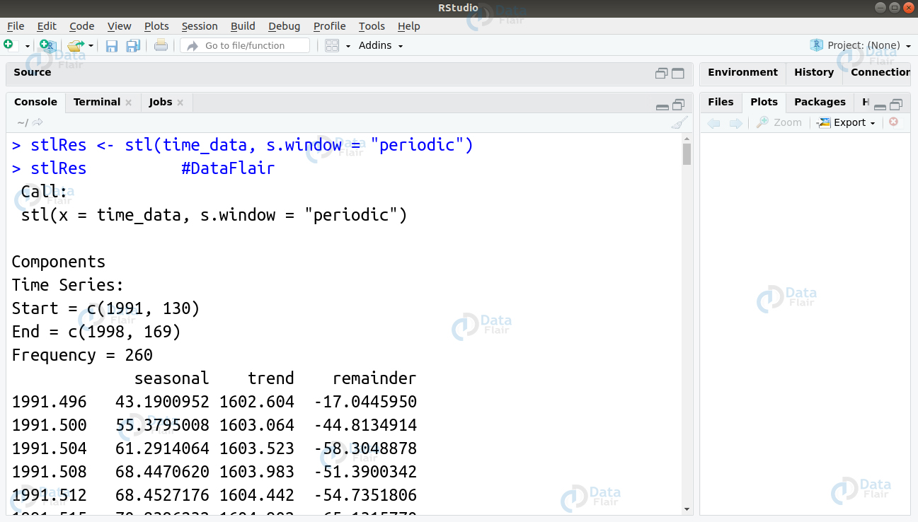
We can also use the stl() function as follows –

> stlRes <- stl(time_data, s.window = "periodic") 
> stlRes #DataFlair

Q.22 You had mentioned White Noise in your previous explanation of stationary time-series analysis. How will you simulate White Noise in R?

Ans. The white noise model is an elementary time-series model. It is a type of stationary process.
The white noise model consists of:

• A fixed constant mean
• A fixed constant variance
• Lack of correlation over time.

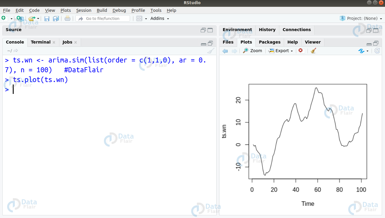
We can simulate a white noise model in R as follows:

> ts.wn <- arima.sim(list(order = c(1,1,0), ar = 0.7), n = 100) #DataFlair
> ts.plot(ts.wn)

Q.23 Explain the differences between Autocorrelation and Partial Correlation by giving an implementation example of each.

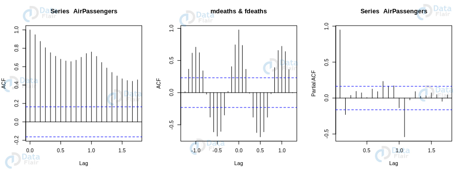
Ans. The correlation of a Time Series model with the delays of itself. It is an important metric due to the following reasons –

• Autocorrelation informs us if the previous states have any form of influence on the current state. If the autocorrelation ranges over the blue line, then we find that particular lag shares some correlation with the present series. For example, in the case of the chart of AirPassengers, we find that the top-left chart exhibits significant autocorrelation for the lags that are depicted on the x-axis.
• We use it for determining of the time-series has a stationary nature or not. A Stationary time-series will cause the autocorrelation to fall to 0 quickly and gradually for a non-stationary series.

In the case of a partial correlation, the time-series has a correlation with its own lag. This takes place with the linear dependence of all the tags removed between them.

We can implement the autocorrelation as well as partial correlation plot as follows –

> par(mfrow = c(1,3))
> autocorr <- acf(AirPassengers) #Autocorrelation
> partialcorr <- pacf(AirPassengers)
> crosscorr <- ccf(mdeaths, fdeaths, ylab = "cross-correlation") #DataFlair
> head(crosscorr[[1]])

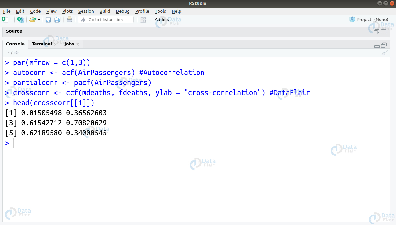
We obtain the following plots that are a result of our above-written code –

R Programming Interview Questions

Q.24 What do you mean by deseasonalizing a time-series. How can you implement this in R?

Ans. In order to gain insights about the time series model, we make use of deseasonalizing. It helps to model our data without causing any seasonal effects.

We can deseasonalize a time-series model in the following steps:

• Decomposing the time-series using forecast::stl() function.
• Using seasadj() function from the forecast package.

Using the seasadj package, one can adjust the seasoning by removing the seasoning components.

library(forecast)
library(ggplot2)
data_decomp <- stl(log(AirPassengers), s.window="periodic")
ap.sea <- exp(seasadj(data_decomp))
autoplot(cbind(AirPassengers, SeasonallyAdjusted=ap.sea)) +
xlab("Year") + ylab("Number of passengers in thousands")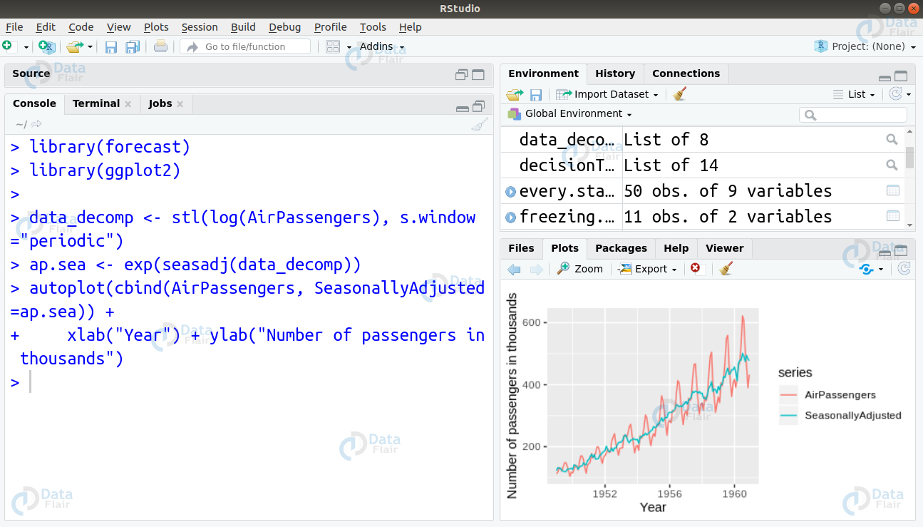

Q.25 What will be the result of this following code:

withCallingHandlers( # (1)
    message = function(dnc) message("d"),
    withCallingHandlers( # (2)
      message = function(dnc) message("c"),
      message(“a”)
    )
)

Ans. When the message(“a”) is run, it is caught by (1). It then places the call to the message (“c”) which in turn gets caught by (2) eventually calling the message (“d”). Since message(“d”) isn’t caught, we see ‘d c’ on the output. This is followed by ‘a’. We get another ‘d’ before we obtain ‘a’ because we have not handled the message. Therefore, it comes up to the outer calling handler.

Q.26 What is a generalized linear model? How can you implement this in R?

Ans. An extension of Linear Regression is the Generalized Linear Models. They allow the dependent variable to be far from normal. There are three assumptions that a general model makes.

• Residuals are mutually independent. Residuals are independent of each other.
• They have normal distribution.
• The parameters x and y of the model possess a linear relationship.

A Generalized Linear Model creates an extension of the last two assumptions. The generalization of the possible distributions that residuals share are to a family called exponential family.

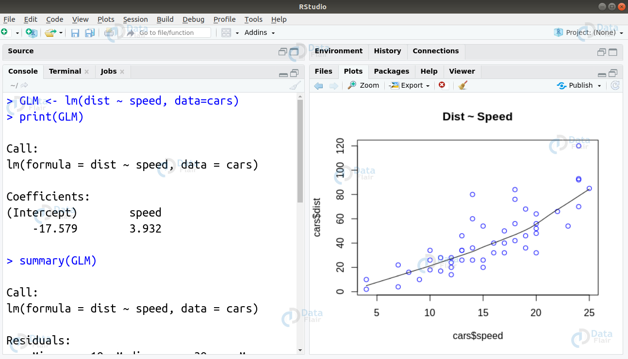
We can implement Generalized Linear Model in R using the lm() function as follows –

#Author DataFlair
data(cars)
head(cars)

scatter.smooth(x=cars$speed, y=cars$dist, main="Dist ~ Speed", col = "blue")

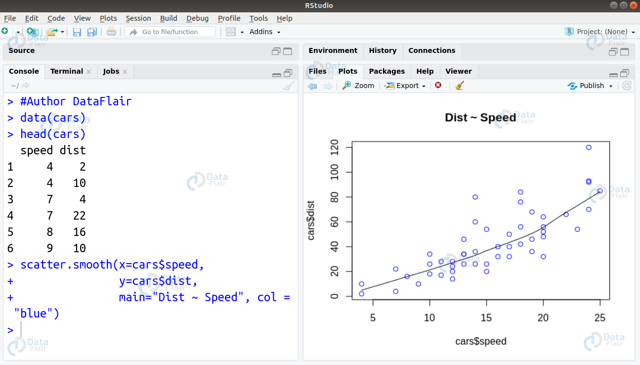
GLM <- lm(dist ~ speed, data=cars)
print(GLM)
summary(GLM)

Q.27 What is a Random Forest algorithm? How can you build an evaluate Random Forest in R?

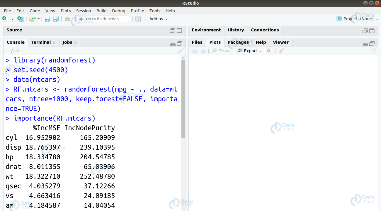
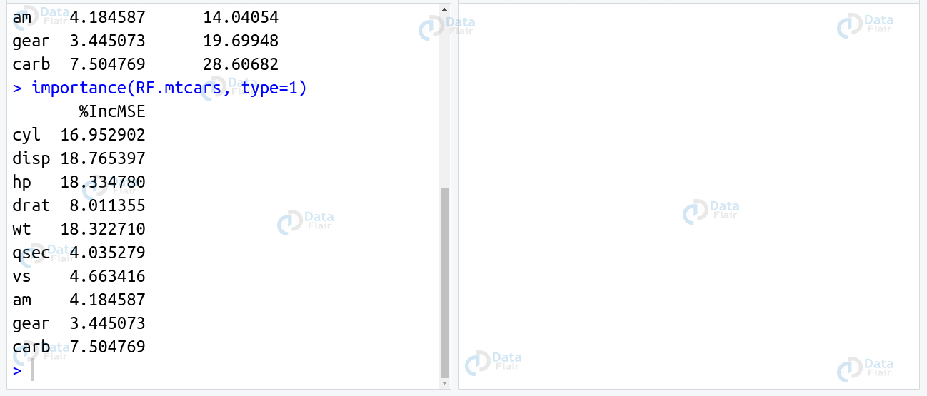
Ans. These are a type of ensemble learning methods that we can use for classification as well as regression. Furthermore, Random Forests perform these tasks using the underlying decision trees. The model constructs them during training time to display the output which can be classification or regression. We can implement our random forest in R using the randomForest package as follows –

library(randomForest)
set.seed(4500)
data(mtcars)
RF.mtcars <- randomForest(mpg ~ ., data=mtcars, ntree=1000, keep.forest=FALSE, importance=TRUE)
importance(RF.mtcars)
importance(RF.mtcars, type=1)

Q.28 What is Ward’s Hierarchical Clustering? Implement this in R using the USArrests dataset.

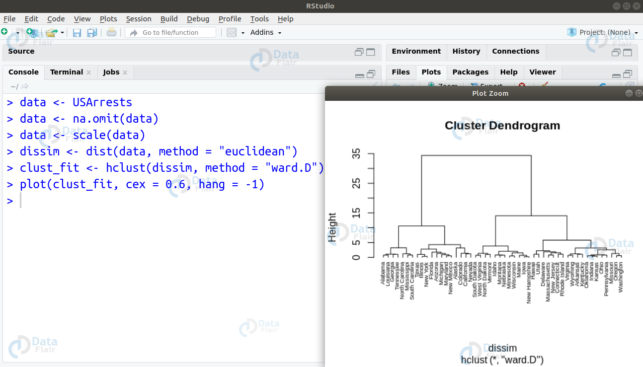
Ans. We use Ward’s method for hierarchical cluster analysis. Its minimum variance method is a special case of the objective function approach. In this, we make use of a general agglomerative hierarchical clustering approach in which the criterion for selecting pair of clusters combine at each step based on the ideal value of the objective function. We can implement this algorithm as follows –

data <- USArrests
data <- na.omit(data)
data <- scale(data)
dissim <- dist(data, method = "euclidean")
clust_fit <- hclust(dissim, method = "ward.D")
plot(clust_fit, cex = 0.6, hang = -1)

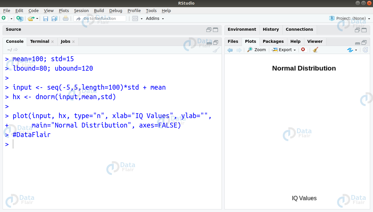
Q.29 Suppose in a survey, IQ scores of school children were measured. The IQ scores were distributed with a mean of 100 and a standard deviation of 15. You want to find the proportion of children having IQ between 80 and 120. How can you solve this using R?

Ans. We can solve this problem by writing the following code to create visualisation of the normal graph as follows –

> mean=100; std=15
> lbound=80; ubound=120
>
> input <- seq(-5,5,length=100)*std + mean
> hx <- dnorm(input,mean,std)
>
> plot(input, hx, type="n", xlab="IQ Values", ylab="",
+      main="Normal Distribution", axes=FALSE)

> i <- input >= lbound & input <= ubound
> lines(input, hx)
> polygon(c(lbound,input[i],ubound), c(0,hx[i],0), col="red")
>
> area <- pnorm(ubound, mean, std) - pnorm(lbound, mean, std)
> result <- paste("P(",lbound,"< IQ <",ubound,") =",
+                 signif(area, digits=3))
> mtext(result,3)
> axis(1, at=seq(40, 160, 20), pos=0)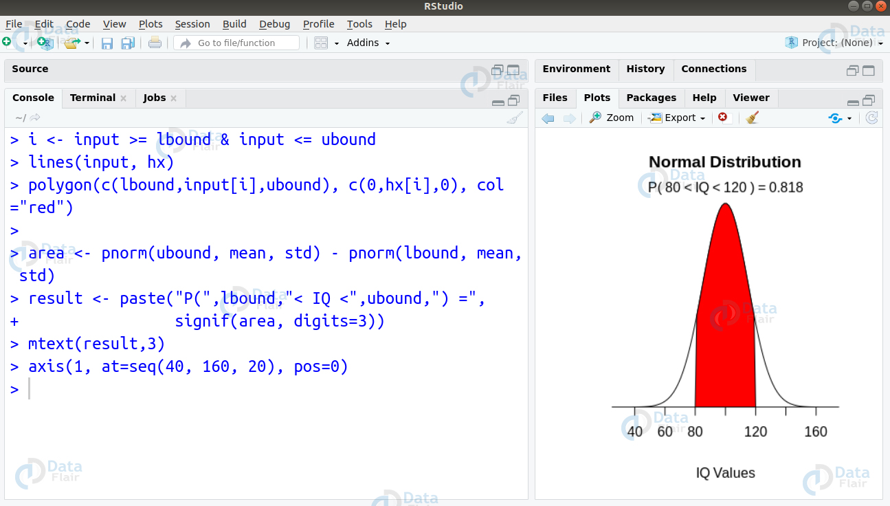

Q.30 How will you carry out bootstrapping of a single statistic (k = 1) in R? Take the example of the mtcars dataset and further replicate the confidence interval by 1000.

Ans. We can perform the bootstrapping of a single statistic by replicating the confidence interval by 10000 as follows –

library(boot)
# function to obtain R-Squared from the data
rsquared <- function(formula, data, indices) {
    dsample <- data[indices,] #Selecting sample
    model.fit <- lm(formula, data=dsample)
    return(summary(fit)$r.square)
}
# Performing bootstrap with 1000 replications
output <- boot(data=mtcars, statistic=rsq,
+               R=1000, formula=mpg~wt+disp)

# view output
output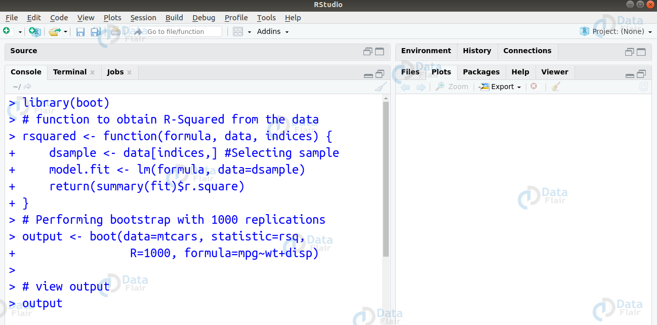

R programming interview questions

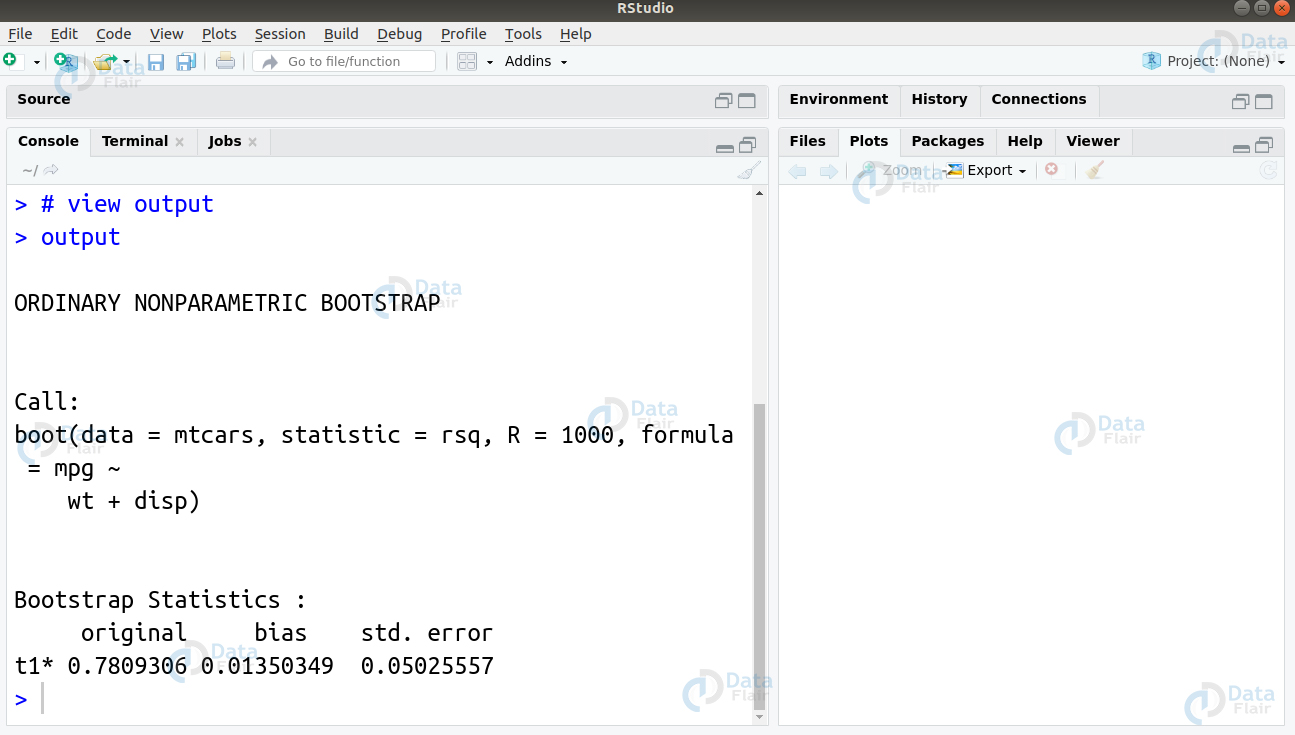
Bootstrapping – R programming interview questions

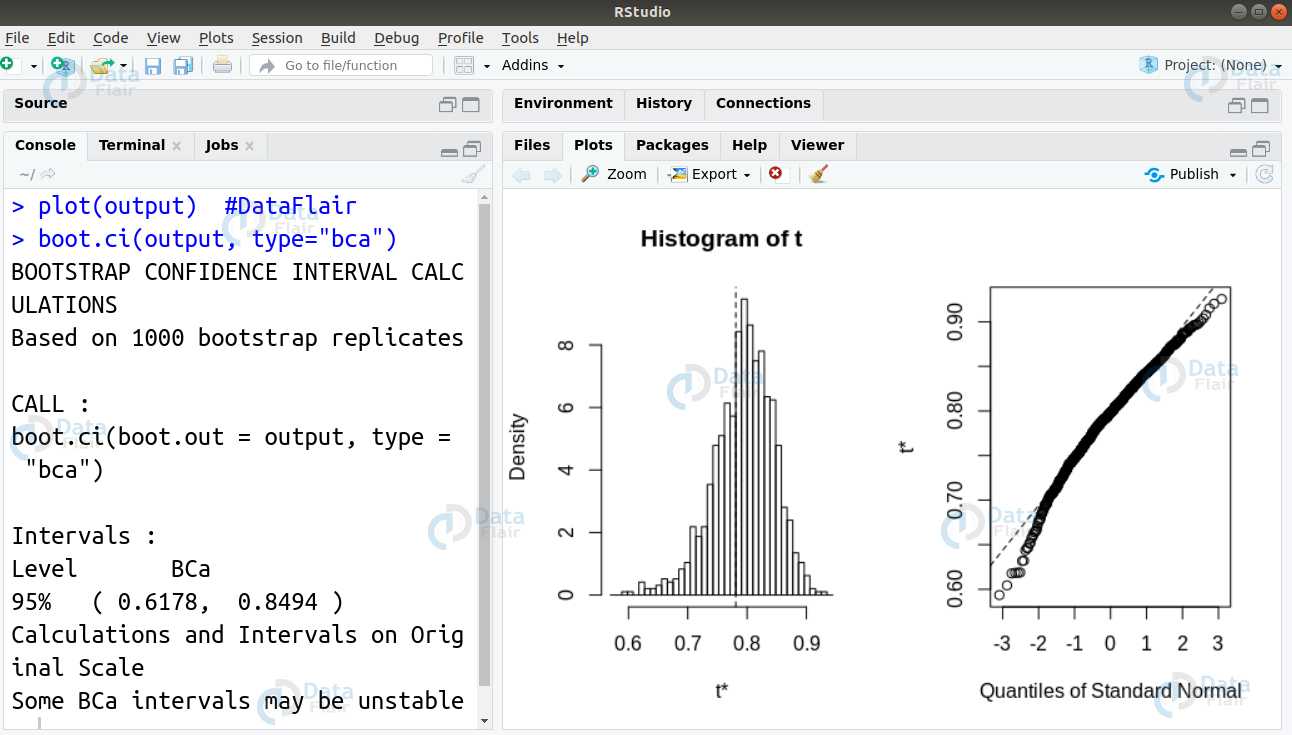
Now, we proceed ahead to plot our output and display our confidence interval as follows

plot(output)
boot.ci(output, type="bca")

I hope after practicing the above R programming interview questions and answers now you are more confident to face your next data science interview.

Are there any R programming interview questions in which you faced difficulty? If yes. then comment below. DataFlair is ready to help you.