Introduction to Hypothesis Testing in R – Learn every concept from Scratch!
Expert-led Online Courses: Elevate Your Skills, Get ready for Future - Enroll Now!
This tutorial is all about hypothesis testing in R. First, we will introduce you with the statistical hypothesis in R, subsequently, we will cover the decision error in R, one and two-sample t-test, μ-test, correlation and covariance in R, etc.
Introduction to Statistical Hypothesis Testing in R
A statistical hypothesis is an assumption made by the researcher about the data of the population collected for any experiment. It is not mandatory for this assumption to be true every time. Hypothesis testing, in a way, is a formal process of validating the hypothesis made by the researcher.
In order to validate a hypothesis, it will consider the entire population into account. However, this is not possible practically. Thus, to validate a hypothesis, it will use random samples from a population. On the basis of the result from testing over the sample data, it either selects or rejects the hypothesis.
Statistical Hypothesis Testing can be categorized into two types as below:
- Null Hypothesis – Hypothesis testing is carried out in order to test the validity of a claim or assumption that is made about the larger population. This claim that involves attributes to the trial is known as the Null Hypothesis. The null hypothesis testing is denoted by H0.
- Alternative Hypothesis – An alternative hypothesis would be considered valid if the null hypothesis is fallacious. The evidence that is present in the trial is basically the data and the statistical computations that accompany it. The alternative hypothesis testing is denoted by H1or Ha.
Let’s take an example of the coin. We want to conclude that a coin is unbiased or not. Since null hypothesis refers to the natural state of an event, thus, according to the null hypothesis, there would an equal number of occurrences of heads and tails, if a coin is tossed several times. On the other hand, the alternative hypothesis negates the null hypothesis and refers that the occurrences of heads and tails would have significant differences in number.
Wait! Have you checked – R Performance Tuning Techniques
Hypothesis Testing in R
Statisticians use hypothesis testing to formally check whether the hypothesis is accepted or rejected. Hypothesis testing is conducted in the following manner:
- State the Hypotheses – Stating the null and alternative hypotheses.
- Formulate an Analysis Plan – The formulation of an analysis plan is a crucial step in this stage.
- Analyze Sample Data – Calculation and interpretation of the test statistic, as described in the analysis plan.
- Interpret Results – Application of the decision rule described in the analysis plan.
Hypothesis testing ultimately uses a p-value to weigh the strength of the evidence or in other words what the data are about the population. The p-value ranges between 0 and 1. It can be interpreted in the following way:
- A small p-value (typically ≤ 0.05) indicates strong evidence against the null hypothesis, so you reject it.
- A large p-value (> 0.05) indicates weak evidence against the null hypothesis, so you fail to reject it.
A p-value very close to the cutoff (0.05) is considered to be marginal and could go either way.
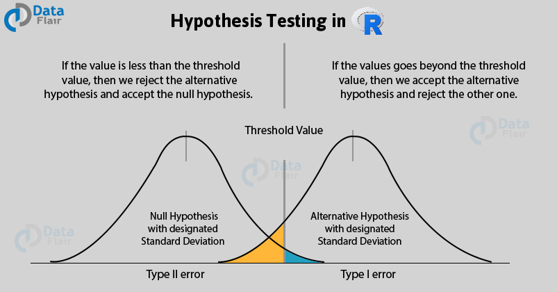
Decision Errors in R
The two types of error that can occur from the hypothesis testing:
- Type I Error – Type I error occurs when the researcher rejects a null hypothesis when it is true. The term significance level is used to express the probability of Type I error while testing the hypothesis. The significance level is represented by the symbol α (alpha).
- Type II Error – Accepting a false null hypothesis H0 is referred to as the Type II error. The term power of the test is used to express the probability of Type II error while testing hypothesis. The power of the test is represented by the symbol β (beta).
Using the Student’s T-test in R
The Student’s T-test is a method for comparing two samples. It can be implemented to determine whether the samples are different. This is a parametric test, and the data should be normally distributed.
R can handle the various versions of T-test using the t.test() command. The test can be used to deal with two- and one-sample tests as well as paired tests.
Listed below are the commands used in the Student’s t-test and their explanation:
- t.test(data.1, data.2) – The basic method of applying a t-test is to compare two vectors of numeric data.
- var.equal = FALSE – If the var.equal instruction is set to TRUE, the variance is considered to be equal and the standard test is carried out. If the instruction is set to FALSE (the default), the variance is considered unequal and the Welch two-sample test is carried out.
- mu = 0 – If a one-sample test is carried out, mu indicates the mean against which the sample should be tested.
- alternative = “two.sided” – It sets the alternative hypothesis. The default value for this is “two.sided” but a greater or lesser value can also be assigned. You can abbreviate the instruction.
- conf.level = 0.95 – It sets the confidence level of the interval (default = 0.95).
- paired = FALSE – If set to TRUE, a matched pair T-test is carried out.
- t.test(y ~ x, data, subset) – The required data can be specified as a formula of the form response ~ predictor. In this case, the data should be named and a subset of the predictor variable can be specified.
- subset = predictor %in% c(“sample.1”, sample.2”) – If the data is in the form response ~ predictor, the two samples to be selected from the predictor should be specified by the subset instruction from the column of the data.
Two-Sample T-test with Unequal Variance
The t.test() command is generally used to compare two vectors of numeric values. The vectors can be specified in a variety of ways, depending on how your data objects are set out.
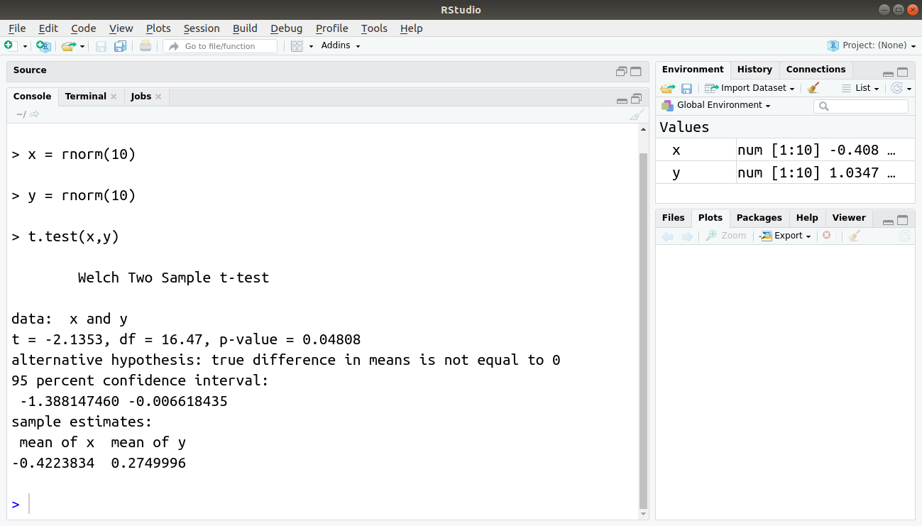
The default form of the t.test() command does not assume that the samples have equal variance. As a result, the two-sample test is carried out unless specified otherwise. The two-sample test can be on any two datasets using the following command:
#Author DataFlair
x = rnorm(10)
y = rnorm(10)
t.test(x,y)
Output:
The default clause in the t.test() command can be overridden. To do so, add the var.equal = TRUE. This is an instruction that is added to the t.test() command. This instruction forces the t.test() command to assume that the variance of the two samples is equal.
The magnitude of the degree of freedom is unmodified as well as the calculations of t-value makes use of the pooled variance.
As a result, the p-value is slightly different from the Welch version. For example:
t.test(x, y, var.equal = TRUE)
Output:
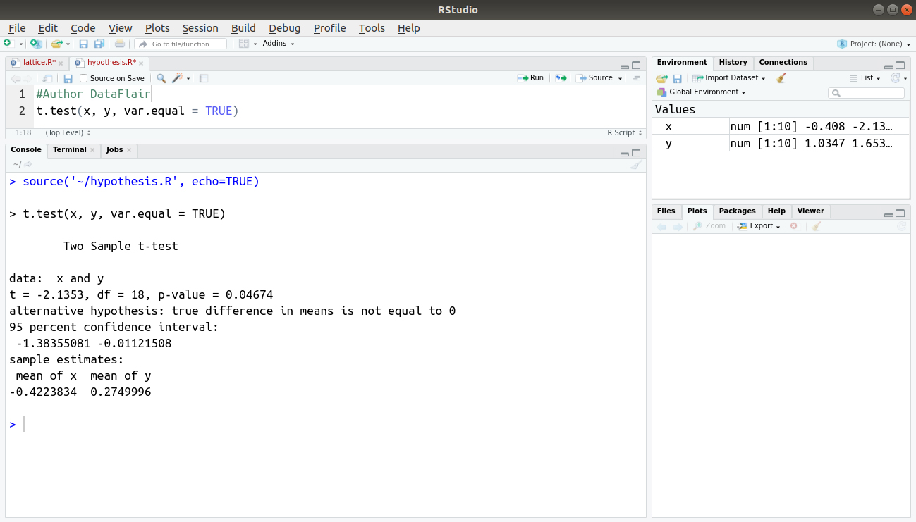
As per the samples estimate, the default clause in the t.test() command can be overridden. To do so, add the var.equal = TRUE instruction to the standard t.test() command. This instruction forces the t.test() command to assume that the variance of the two samples is equal.
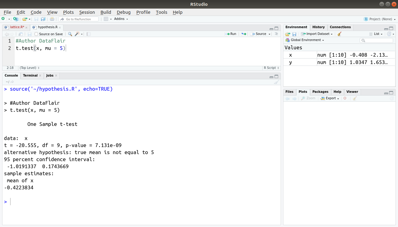
One-Sample T-testing in R
To perform analysis, it collects a large amount of data from various sources and tests it on random samples. In several situations, when the population of collected data is unknown, researchers test samples to identify the population. The one-sample T-test is one of the useful tests for testing the sample’s population.
This test is used for testing the mean of samples. For example, you can use this test to compare that a sample of students from a particular college is identical or different from the sample of general students. In this situation, the hypothesis tests that the sample is from a known population with a known mean (m) or from an unknown population.
To carry out a one-sample T-test in R, the name of a single vector and the mean with which it is compared is supplied.
The mean defaults to 0.
The one-sample T-test can be implemented as follows:
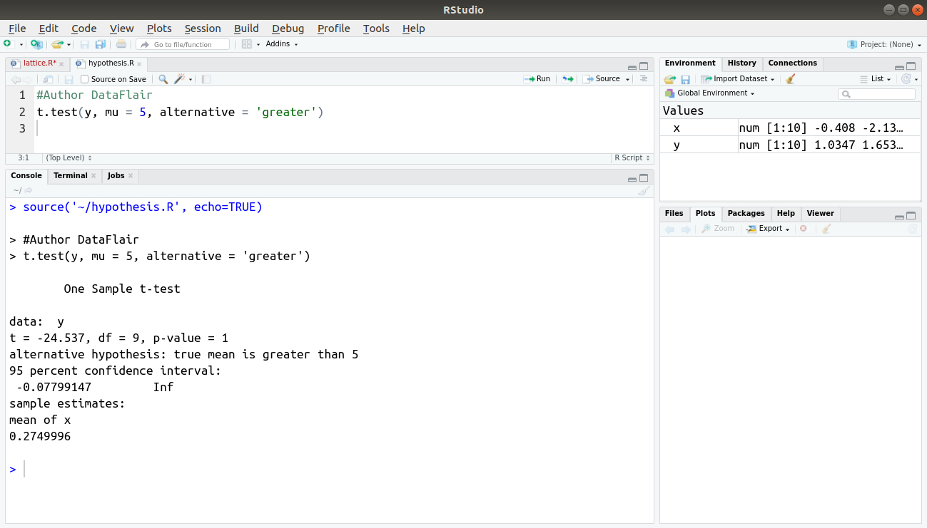
#Author DataFlair
t.test(x, mu = 5)
Output:
Learn to perform T-tests in R and master the concept
Using Directional Hypotheses in R
You can also specify a “direction” to your hypothesis.
In many cases, you are simply testing to see if the means of two samples are different, but you may want to know if a sample mean is lower or greater than another sample mean. You can use the alternative equal to (=) instruction to switch the emphasis from a two-sided test (the default) to a one-sided test. The choices you have are between ″two.sided″, ″less″, or ″greater″, and the choice can be abbreviated, as shown in the following command:
#Author DataFlair
t.test(y, mu = 5, alternative = 'greater')
Output:
Formula Syntax and Subsetting Samples in the T-test in R
As discussed in the previous sections, the T-test is designed to compare two samples.
So far, we have seen how to carry out the T-test on separate vectors of values; however, your data may be in a more structured form with a column for the response variable and a column for the predictor variable.
When the data is available in a more structured form with a separate column for the response variable and predictor variable, the data can be set in a more sensible and flexible manner. You need a new way to deal with the layout.
R deals with the layout by using a formula syntax.
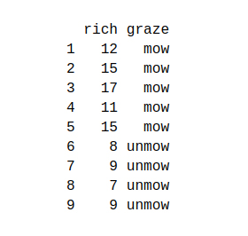
In this section, we will use the grass dataset:
You can download the dataset from here – Grass Dataset
You can create a formula by using the tilde (~) symbol. Essentially, your response variable goes to the left of the ~ and the predictor goes to the right, as shown in the following command:
> t.test(rich ~ graze, data = grass)
If your predictor column contains more than two items, the T-test cannot be used; however, you can still carry out a test by subsetting this predictor column and specifying the two samples you want to compare.
The subset = instruction should be used as a part of the t.test() command, as follows:
Formula Syntax in R – The following example illustrates how to do this using the same data as in the previous example:
> t.test(rich ~ graze, data = grass, subset = graze %in% c('mow‘, 'unmow'))Output:
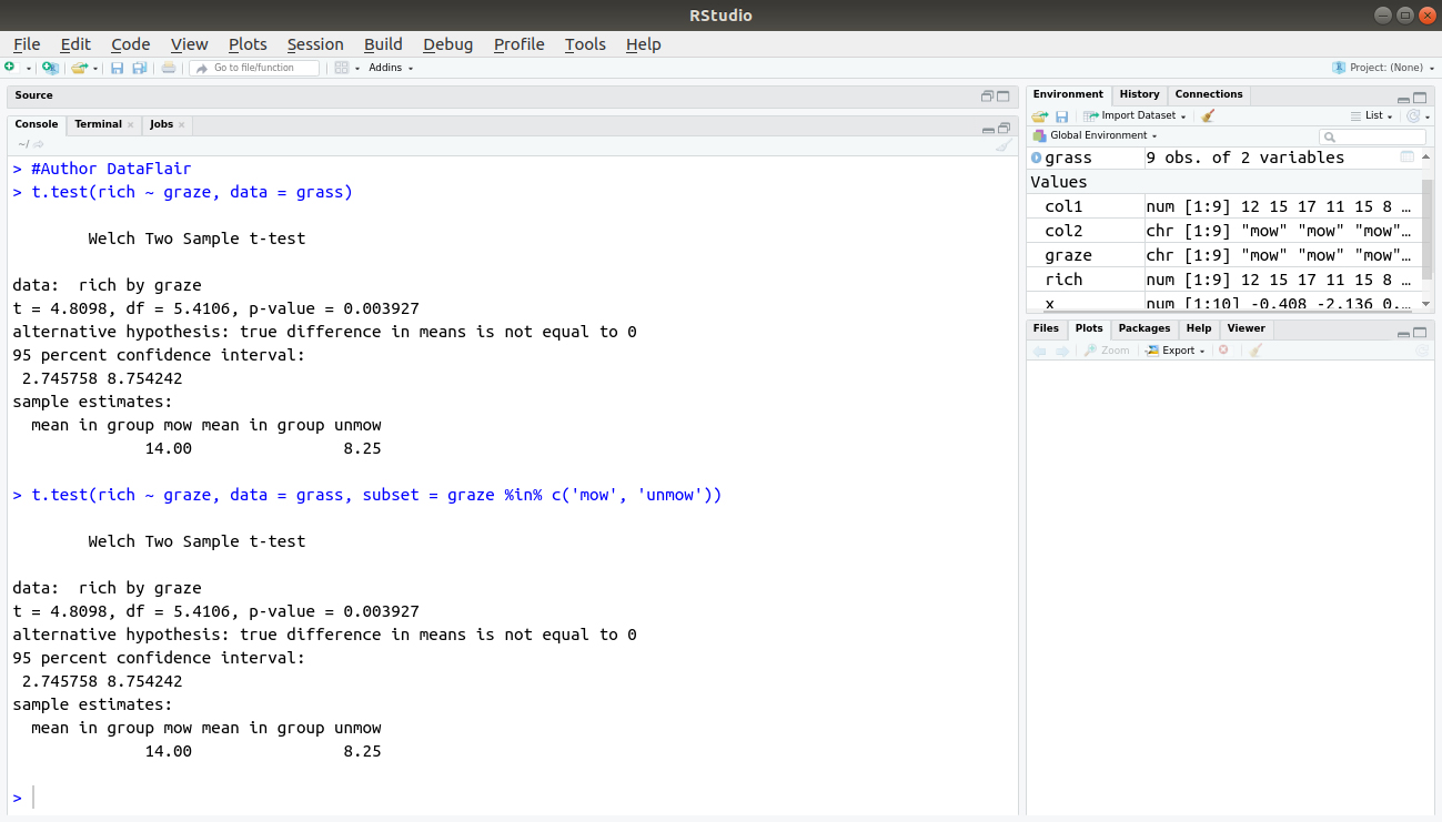
You first specify the column from which you want to take your subset and then type %in%. This tells the command that the list that follows is in the graze column. Note that, you have to put the levels in quotes; here you compare ″mow″and ″unmow″and your result is identical to the one you obtained before.
μ-test in R
When you have two samples to compare and your data is nonparametric, you can use the μ-test. This goes by various names and may be known as the Mann—Whitney μ-test or Wilcoxon sign rank test. The wilcox.test() command can carry out the analysis.
The wilcox.test() command can conduct two-sample or one-sample tests, and you can add a variety of instructions to carry out the test.
Given below are the main options available in the wilcox.test() command with their explanation:
- test(sample.1, sample.2) – It carries out a basic two-sample μ-test on the numerical vectors specified.
- mu = 0 – If a one-sample test is carried out, mu indicates the value against which the sample should be tested.
- alternative = “two.sided” – It sets the alternative hypothesis. “two.sided” is the default value, but a greater or lesser value can also be assigned. You can abbreviate the instruction but you still need the quotes.
- int = FALSE – It sets whether confidence intervals should be reported or not.
- level = 0.95 – It sets the confidence level of the interval (default = 0.95).
- correct = TRUE – By default, the continuity correction is applied. This can also be set to FALSE.
- paired = FALSE – If set to TRUE, a matched pair μ-test is carried out.
- exact = NULL – It sets whether an exact p-value should be computed. The default is to do so for less than 50 items.
- test(y ~ x, data, subset) – The required data can be specified as a formula of the form response ~ predictor. In this case, the data should be named and a subset of the predictor variable can be specified.
- subset = predictor %in% c(″1″, ″sample.2″) – If the data is in the form response ~ predictor, the subset instruction can specify the two samples to select from the predictor column of the data.
Don’t forget to check the R Vector Functions
Two-Sample μ-test in R
The basic way of using wilcox.test() command is to specify the two samples you want to compare as separate vectors, as shown in the following command:
> x ; y
> wilcox.test(x, y)
Output:
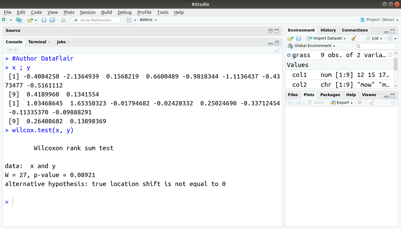
By default, the confidence intervals are not calculated and the p-value is adjusted using the “continuity correction”; a message tells you that the latter has been used. In this case, you see a warning message because you have tied values in the data. If you set exact = FALSE, this message would not be displayed because the p-value would be determined from a normal approximation method.
Any doubts in Hypothesis Testing in R, till now? Share your queries in the comment section.
One-Sample μ-test in R
When you specify a single numerical vector, then it carries out a one-sample μ-test. The default is to set mu = 0. For example:
> #Author DataFlair
> wilcox.test(y, exact = FALSE)
Output:
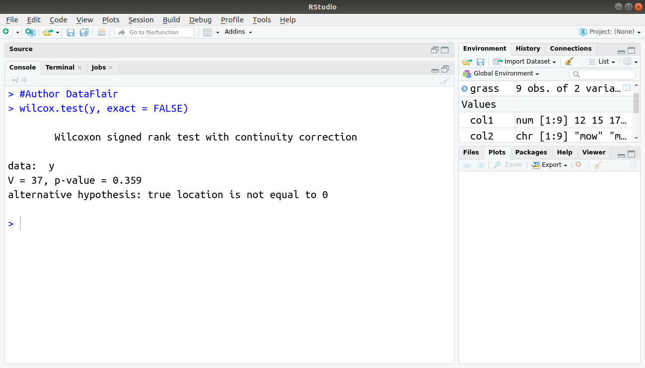
In this case, the p-value is a normal approximation because it uses the exact = FALSE instruction. The command has assumed mu = 0 because it is not specified explicitly.
Formula Syntax and Subsetting Samples in the μ-test in R
It is better to have data arranged into a data frame where one column represents the response variable and another represents the predictor variable. In this case, the formula syntax can be used to describe the situation and carry out the wilcox.test() command on your data. The method is similar to what is used for the T-test.
The basic form of the command is:
wilcox.test(response ~ predictor, data = my.data)
You can also use additional instructions as you could with the other syntax. If the predictor variable contains more than two samples, you cannot conduct a μ-test and use a subset that contains exactly two samples.
Notice that in the preceding command, the names of the samples must be specified in quotes in order to group them together. The μ-test is one of the most widely used statistical methods, so it is important to be comfortable in using the wilcox.test()command. In the following activity, you try conducting a range of μ-tests for yourself. The μ-test is a useful tool for comparing two samples and is one of the most widely used tools of all simple statistical tests. Both the t.test()and wilcox.test()commands can also deal with matched-pair data.
Correlation and Covariance in R
When you have two continuous variables, you can look for a link between them. This link is called a correlation.
The cor() command determines correlations between two vectors, all the columns of a data frame, or two data frames. The cov() command examines covariance. The cor.test() command carries out a test of significance of the correlation.
You can add a variety of additional instructions to these commands, as given below:
- cor(x, y = NULL) – It carries out a basic correlation between x and y. If x is a matrix or data frame, we can omit y. One can correlate any object against any other object as long as the length of the individual vectors matches up.
- cov(x, y = NULL) – It determines covariance between x and y. If x is a matrix or data frame, one can omit y.
- cov2cor(V) – It takes a covariance matrix V and calculates the correlation.
- method = – The default is “pearson”, but “spearman” or “kendall” can be specified as the methods for correlation or covariance. These can be abbreviated but you still need the quotes and note that they are lowercase.
- var(x, y = NULL) – It determines the variance of x. If x is a matrix or data frame and y is specified, it also determines the covariance.
- test(x, y) – It carries out a significance test of the correlation between x and y. In this case, you can now specify only two data vectors, but you can use a formula syntax, which makes it easier when the variables are within a data frame or matrix. The Pearson product-moment is the default, but it can also use Spearman’s Rho or Kendall’s Tau tests. You can use the subset command to select data on the basis of a grouping variable.
- alternative = “two.sided” – The default is for a two-sided test but the alternative hypothesis can be given as “two.sided”, “greater”, or “less”.
- level = 0.95 – If the method = “pearson” and n > 3, it will show the confidence intervals. This instruction sets the confidence level and defaults to 0.95.
A concept to ease your journey of R programming – R Data Frame
Simple Correlation in R
Simple correlations are between two continuous variables and use the cor() command to obtain a correlation coefficient, as shown in the following command:
#Author DataFlair
count = c(9,25,15,2,14,25,24,47)
speed = c(2,3,5,9,14,24,29,34)
cor(count, speed)
cor(count, speed, method = 'spearman')
Output:
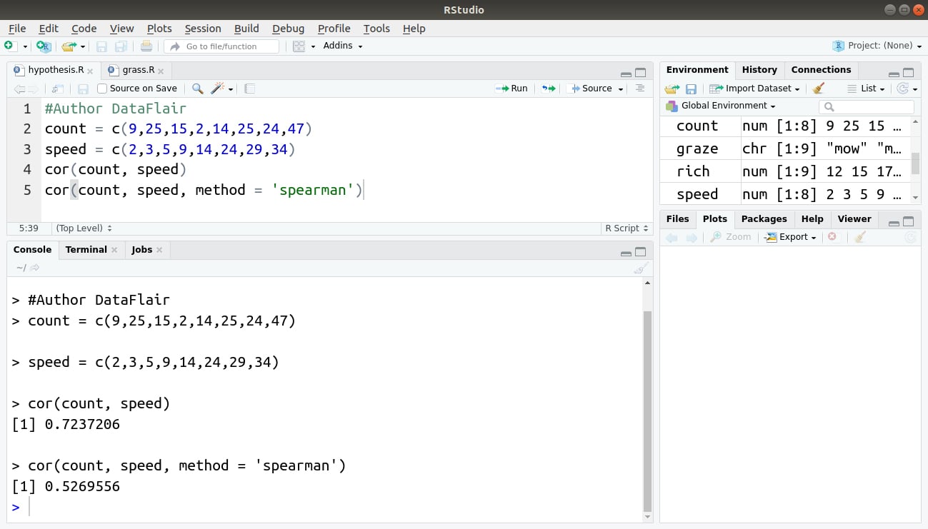
This example used the Spearman Rho correlation but you can also apply Kendall’s tau by specifying method = ″kendall″. Note that you can abbreviate this but you still need the quotes. You also have to use lowercase.
If your vectors are within a data frame or some other object, you need to extract them in a different fashion.
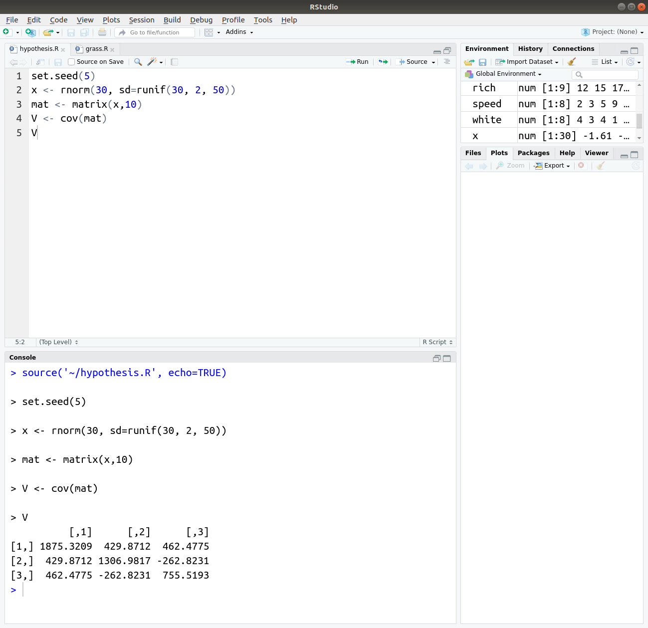
Covariance in R
The cov() command uses syntax similar to the cor() command to examine covariance.
We can use the cov() command as:
set.seed(5)
x <- rnorm(30, sd=runif(30, 2, 50))
mat <- matrix(x,10)
V <- cov(mat)
V
Output:
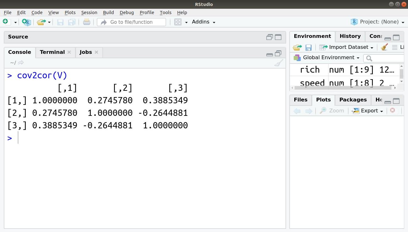
The cov2cor() command determines the correlation from a matrix of covariance, as shown in the following command:
> cov2cor(V)
Output:
Significance Testing in Correlation Tests
You can apply a significance test to your correlations by using the cor.test() command. In this case, you can compare only two vectors at a time, as shown in the following command:
> #DataFlair
> cor.test(women$height, women$weight)
Output:
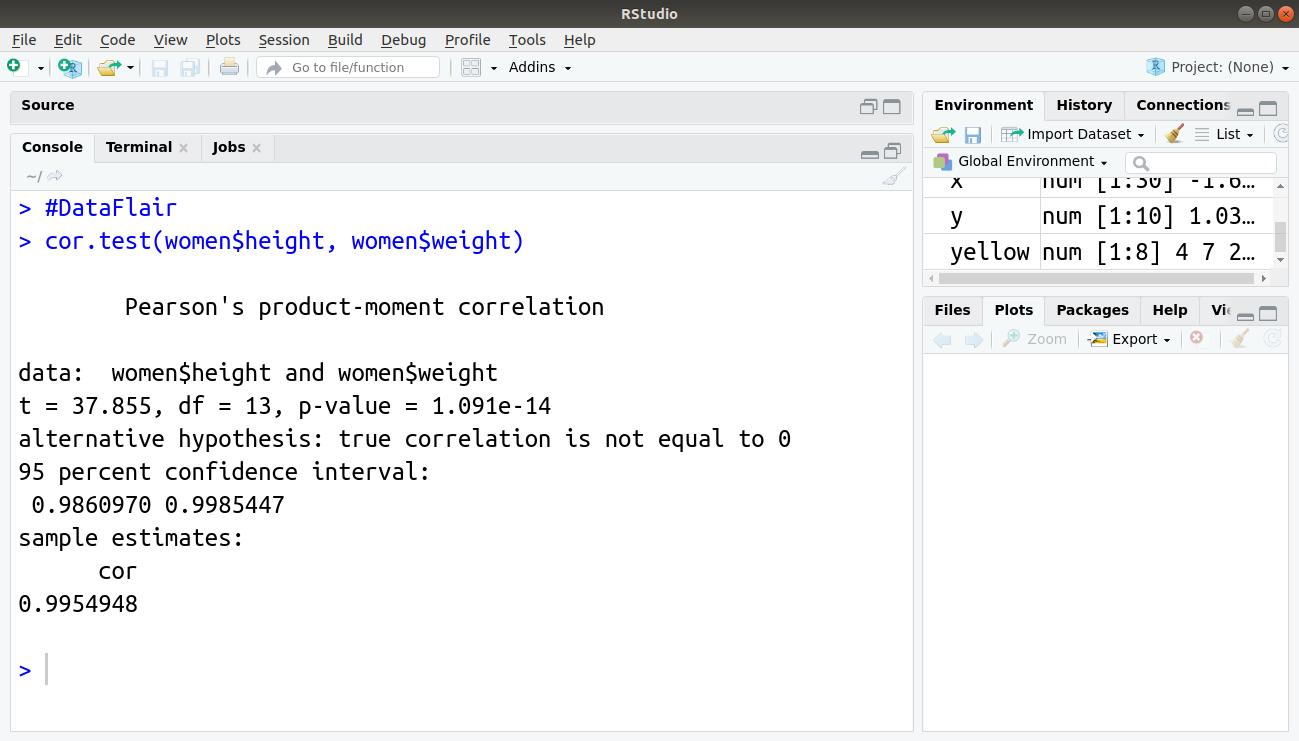
In the previous example, you can see that the Pearson correlation is between height and weight in the data of women and the result also shows the statistical significance of the correlation.
You must definitely learn about Descriptive Statistics in R
Formula Syntax in R
If your data is in a data frame, using the attach() or with() command is tedious, as is using the $ syntax. A formula syntax is available as an alternative, which provides a neater representation of your data, as shown in the following command:
> data(cars)
> cor.test(~ speed + dist, data = cars, method = 'spearman', exact = F)
Output:
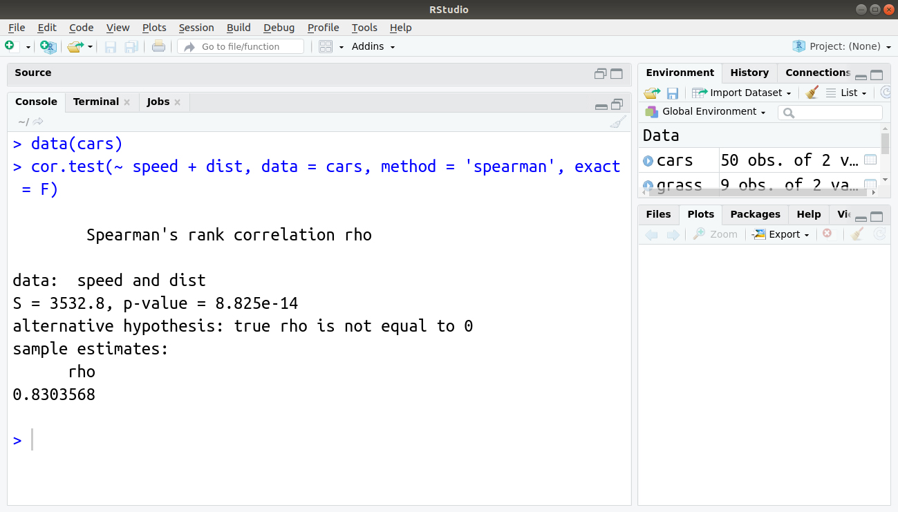
Here you examine the data of cars, which comes built-in in R. The formula is slightly different from the one that you used previously. Here you specify both variables to the right of the ~. You also give the name of the data as a separate instruction. All the additional instructions are available while using the formula syntax as well as the subset instruction.
Tests for Association in R
When you have categorical data, you can look for associations between categories by using the chi-squared test. Routines to achieve this is possible by using the chisq.test() command.
The various additional instructions that you can add to the chisq.test() command are:
- test(x, y = NULL) – A basic chi-squared test is carried out on a matrix or data frame. If it provides x as a vector, a second vector can be supplied. If x is a single vector and y is not given, a goodness of fit test is carried out.
- correct = TRUE – It applies Yates’ correction if the data forms a 2 n 2 contingency table.
- p = – It is a vector of probabilities for use with a goodness of fit test. If p is not given, the goodness of fit tests that the probabilities are all equal.
- p = FALSE – If TRUE, p is rescaled to sum to 1. For use with the goodness of fit tests.
- p.value = FALSE – If set to TRUE, a Monte Carlo simulation calculates p-values.
- B = 2000 – The number of replicates to use in the Monte Carlo simulation.
Get a deep insight into Contingency Tables in R
Goodness of Fit Tests in R
While fitting a statistical model for observed data, an analyst must identify how accurately the model analysis the data. This is done with the help of the chi-square test.
The chi-square test is a type of hypothesis testing methodology that identifies the goodness-of-fit by testing whether the observed data is taken from the claimed distribution or not. The two values included in this test are observed value, the frequency of a category from the sample data, and expected frequency that is calculated on the basis of an expected distribution of the sample population. The chisq.test() command can be used to carry out the goodness of fit test.
In this case, you must have two vectors of numerical values, one representing the observed values and the other representing the expected ratio of values. The goodness of fit tests the data against the ratios you specified. If you do not specify any, the data is tested against equal probability.
The basic form of the chisq.test() command will operate on a matrix or data frame.
By enclosing the command completely within parentheses, you can get the result object to display immediately. The results of many commands are stored as a list containing several elements, and you can see what is available by using the names() command and view them by using the $syntax.
The p-value can be determined using a Monte Carlo simulation by using the simulate.p.value and B instructions. If the data form a 2 n 2 contingency, then Yates’ correction is automatically applied but only if the Monte Carlo simulation is not used.
To conduct goodness of fit test, you must specify p, the vector of probabilities; if this does not add to 1, you will get an error unless you use rescale.p = TRUE. You can use a Monte Carlo simulation on the goodness of fit test. If a single vector is specified, a goodness of fit test is carried out but the probabilities are assumed to be equal.
Summary
In this article, we studied about Hypothesis testing in R. We learned about the basics of the null hypothesis as well as alternative hypothesis. We read about T-test and μ-test. Then, we implemented these statistical methods in R.
The next tutorial in our R DataFlair tutorial series – R Linear Regression Tutorial
Hope the article was useful for you. In case of any queries related to hypothesis testing in R, please share your views in the comment section below.
Did we exceed your expectations?
If Yes, share your valuable feedback on Google


HI
I Marry CumMaster69