Classification in R Programming: The all in one tutorial to master the concept!
Job-ready Online Courses: Click for Success - Start Now!
In this tutorial, we will study the classification in R thoroughly. We will also cover the Decision Tree, Naïve Bayes Classification and Support Vector Machine. To understand it in the best manner, we will use images and real-time examples.
Introduction to Classification in R
We use it to predict a categorical class label, such as weather: rainy, sunny, cloudy or snowy.
Important points of Classification in R
There are various classifiers available:
- Decision Trees – These are organised in the form of sets of questions and answers in the tree structure.
- Naive Bayes Classifiers – A probabilistic machine learning model that is used for classification.
- K-NN Classifiers – Based on the similarity measures like distance, it classifies new cases.
- Support Vector Machines – It is a non-probabilistic binary linear classifier that builds a model to classify a case into one of the two categories.
An example of classification in R through Support Vector Machine is the usage of classification() function:
classification(trExemplObj,classLabels,valExemplObj=NULL,kf=5,kernel=”linear”)
Wait! Have you completed the tutorial on Clustering in R
Arguments:
1. trExemplObj – It is an exemplars train eSet object.
2. classLabels – It is being stored in eSet object as variable name e.g “type”.
3. valExemplObj – It is known as exemplars validation eSet object.
4. kf – It is termed as the k-folds value of the cross-validation parameter. Also, the default value is 5-folds. By setting “Loo” or “LOO” a Leave-One-Out Cross-Validation which we have to perform.
5. kernel – In classification analysis, we use a type of Kernel. The default kernel is “linear”.
6. classL – The labels of the train set.
7. valClassL – It is termed as the labels of the validation set if not NULL.
8. predLbls – It is defined as the predicted labels according to the classification analysis.
Decision Tree in R
It is a type of supervised learning algorithm. We use it for classification problems. It works for both types of input and output variables. In this technique, we split the population into two or more homogeneous sets. Moreover, it is based on the most significant splitter/differentiator in input variables.
The Decision Tree is a powerful non-linear classifier. A Decision Tree makes use of a tree-like structure to generate relationship among the various features and potential outcomes. It makes use of branching decisions as its core structure.

In classifying data, the Decision Tree follows the steps mentioned below:
- It puts all training examples to a root.
- Based on the various selected attributes, a Decision Tree divides these training examples.
- Then it will select attributes by using some statistical measures.
- Recursive partitioning continues until no training example remains.
1. Important Terminologies related to Decision Tree
- Root Node: It represents the entire population or sample. Moreover, it gets divided into two or more homogeneous sets.
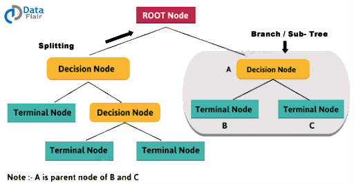
- Splitting: In this, we carry out the division of a node into two or more sub-nodes.
- Decision Tree: It is produced when a sub-node splits into further sub-nodes.
- Leaf/Terminal Node: Nodes that do not split is called Leaf or Terminal node.
- Pruning: When we remove sub-nodes of a decision node, this process is called pruning. It is the opposite process of splitting.
- Branch / Sub-Tree: A subsection of the entire tree is called branch or sub-tree.
- Parent and Child Node: A node, which is divided into sub-nodes is called a parent node of sub-nodes whereas sub-nodes are the child of a parent node.
2. Types of Decision Tree
- Categorical(classification) Variable Decision Tree: Decision Tree which has a categorical target variable.
- Continuous(Regression) Variable Decision Tree: Decision Tree has a continuous target variable.
Don’t forget to check out the R Decision Trees in detail
3. Categorical (classification) Trees vs Continuous (regression) Trees
Regression trees are used when the dependent variable is continuous while classification trees are used when the dependent variable is categorical.
In continuous, a value obtained is a mean response of observation.
In classification, a value obtained by a terminal node is a mode of observations.
There is one similarity in both cases. The splitting process continues results in grown trees until it reaches to stopping criteria. But, the grown tree is likely to overfit data, leading to poor accuracy on unseen data. This brings ‘pruning’. Pruning is one of the techniques which uses tackle overfitting.
4. Advantages of Decision Tree in R
- Easy to Understand: It does not need any statistical knowledge to read and interpret them. Its graphical representation is very intuitive and users can relate their hypothesis.
- Less data cleaning required: Compared to some other modeling techniques, it requires fewer data.
- Data type is not a constraint: It can handle both numerical and categorical variables.
- Simple to understand and interpret.
- Requires little data preparation.
- It works with both numerical and categorical data.
- Handles non-linearity.
- Possible to confirm a model using statistical tests.
- It is robust. It performs well even if you deviate from assumptions.
- It scales to Big Data.
You must definitely explore the R Nonlinear Regression Analysis
Disadvantages of R Decision Tree
- Overfitting: It is one of the most practical difficulties for Decision Tree models. By setting constraints on model parameters and pruning, we can solve this problem in R.
- Not fit for continuous variables: At the time of using continuous numerical variables. Whenever it categorizes variables in different categories, the Decision Tree loses information.
- To learn globally optimal tree is NP-hard, algos rely on greedy search.
- Complex “if-then” relationships between features inflate tree size. Example – XOR gate, multiplexor.
Introduction to Naïve Bayes Classification
We use Bayes’ theorem to make the prediction. It is based on prior knowledge and current evidence.
Bayes’ theorem is expressed by the following equation:

where P(A) and P(B) are the probability of events A and B without regarding each other. P(A|B) is the probability of A conditional on B and P(B|A) is the probability of B conditional on A.
Introduction to Support Vector Machines
What is Support Vector Machine?
We use it to find the optimal hyperplane (line in 2D, a plane in 3D and hyperplane in more than 3 dimensions). Which helps in maximizes the margin between two classes. Support Vectors are observations that support hyperplane on either side.
It helps in solving a linear optimization problem. It also helps out in finding the hyperplane with the largest margin. We use the “Kernel Trick” to separate instances that are inseparable.
Terminologies related to R SVM
Why Hyperplane?
It is a line in 2D and plane in 3D. In higher dimensions (more than 3D), it’s called as a hyperplane. Moreover, SVM helps us to find a hyperplane that can separate two classes.
What is Margin?
A distance between the hyperplane and the closest data point is called a margin. But if we want to double it, then it would be equal to the margin.
How to find the optimal hyperplane?
First, we have to select two hyperplanes. They must separate the data with no points between them. Then maximize the distance between these two hyperplanes. The distance here is ‘margin’.
What is Kernel?
It is a method which helps to make SVM run, in case of non-linear separable data points. We use a kernel function to transforms the data into a higher dimensional feature space. And also with the help of it, perform the linear separation.
Different Kernels
1. linear: u’*v
2. polynomial: (gamma*u’*v + coef0)^degree
3. radial basis (RBF) : exp(-gamma*|u-v|^2)sigmoid : tanh(gamma*u’*v + coef0)
RBF is generally the most popular one.
How SVM works?
- Choose an optimal hyperplane which maximizes margin.
- Applies penalty for misclassifications (cost ‘c’ tuning parameter).
- If the non-linearly separable the data points. Then transform data to high dimensional space. It is done so in order to classify it easily with the help of linear decision surfaces.
Time to master the concept of Data Visualization in R
Advantages of SVM in R
- If we are using Kernel trick in case of non-linear separable data then it performs very well.
- SVM works well in high dimensional space and in case of text or image classification.
- It does not suffer a multicollinearity problem.
Disadvantages of SVM in R
- It takes more time on large-sized data sets.
- SVM does not return probability estimates.
- In the case of linearly separable data, this is almost like logistic regression.
Support Vector Machine – Regression
- Yes, we can use it for a regression problem, wherein the dependent or target variable is continuous.
- The aim of SVM regression is the same as classification problem i.e. to find the largest margin.
Applications of Classification in R
- An emergency room in a hospital measures 17 variables of newly admitted patients. Variables, like blood pressure, age and many more. Furthermore, a careful decision has to be made if the patient has to be admitted to the ICU. Due to a high cost of I.C.U, those patients who may survive more than a month are given high priority. Also, the problem is to predict high-risk patients. And, to discriminate them from low-risk patients.
- A credit company receives hundreds of thousands of applications for new cards. The application contains information about several different attributes. Moreover, the problem is to categorize those who have good credit, bad credit or fall into a grey area.
- Astronomers have been cataloguing distant objects in the sky using long exposure C.C.D images. Thus, the object that needs to be labelled is a star, galaxy etc. The data is noisy, and the images are very faint, hence, the cataloguing can take decades to complete.
Summary
We have studied about classification in R along with their usages and pros and cons. We have also learned real-time examples which help to learn classification in a better way.
Next tutorial in our R DataFlair tutorial series – e1071 Package | SVM Training and Testing Models in R
Still, if any doubts regarding the classification in R, ask in the comment section.
Did we exceed your expectations?
If Yes, share your valuable feedback on Google


Classification is one of the most important algorithms in R. There are several algo for classification: Naive Byes, Decision tree, SVM, etc.
Thanks for sharing this valuable information.
Hii Asif,
Thanks for sharing such valuable information with us. Your review on this blog is appreciable. Keep learning with us.
Data Flair
hi Data flair,
excellent piece of write up here. classification is very important process in R to categorize the data and make decisions. Nicely explained about the same. if some project examples are available that would be great.
How do you analyze a data having ordinal(scale) variable, nominal variable, numeric variable, classified nominal variable
Download the Bachelor’s Degree Graduation Project Ready Book in Artificial Intelligence in the Field of Medicine
Hello, i think the analysis of the K-NN classifier is missing here. I was also wondering, will there be a description of the Discriminant Analysis Classifier? The analysis of the multidimensional scaling and principal component analysis would be also useful. Thank you.