Normal Distribution in R – Implement Functions with the help of Examples!
Job-ready Online Courses: Click, Learn, Succeed, Start Now!
In this tutorial, we will learn about Normal Distribution in R. We will cover different functions which helps in generating the normal distribution. Along with this, we will also include graphs for easy representation and understanding.
Let’s start the tutorial.
What is Normal Distribution in R?
Generally, it is observed that the collection of random data from independent sources is distributed normally. We get a bell shape curve on plotting a graph with the value of the variable on the horizontal axis and the count of the values in the vertical axis. The centre of the curve represents the mean of the dataset.
It has four inbuilt functions. They are described below:
- dnorm()
- qnorm()
- pnorm()
- rnorm()
We use the following functions in the above-stated parameters:
- x is a vector of numbers.
- p is a vector of probabilities.
- n is the number of observations (sample size).
- Here, mean is the mean value of the sample data. Also, its default value is zero.
- sd is the standard deviation. Its default value is 1.
Must Learn – How to apply Functions over R Vectors
Functions to Generate Normal Distribution in R
Below are the different functions to generate normal distribution in R programming:
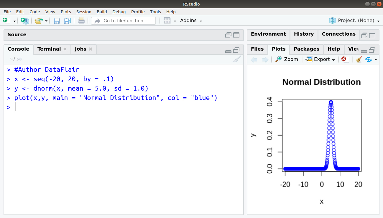
1. dnorm()
Syntax: dnorm(x, mean, sd)
For example:
Create a sequence of numbers between -10 and 10 incrementing by 0.1.
> #Author DataFlair
> x <- seq(-20, 20, by = .1)
> y <- dnorm(x, mean = 5.0, sd = 1.0)
> plot(x,y, main = "Normal Distribution", col = "blue")
Output:
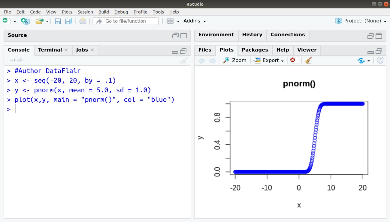
2. pnorm()
Syntax: pnorm(x,mean,sd)
For example:
> #Author DataFlair
> x <- seq(-20, 20, by = .1)
> y <- pnorm(x, mean = 5.0, sd = 1.0)
> plot(x,y, main = "pnorm()", col = "blue")
Output:
You must definitely check the Numeric and Character Functions in R
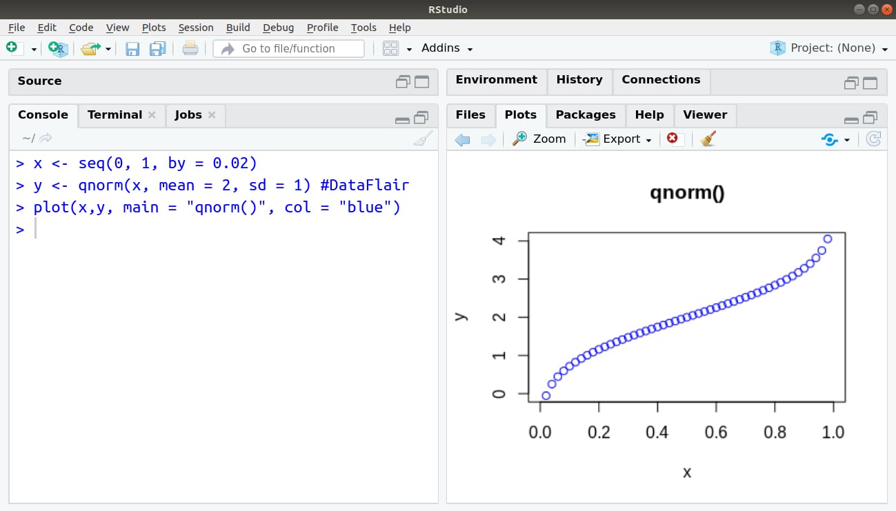
3. qnorm()
Syntax: qnorm(x,mean,sd)
For example:
> x <- seq(0, 1, by = 0.02)
> y <- qnorm(x, mean = 2, sd = 1) #DataFlair
> plot(x,y, main = "qnorm()", col = "blue")
Output:
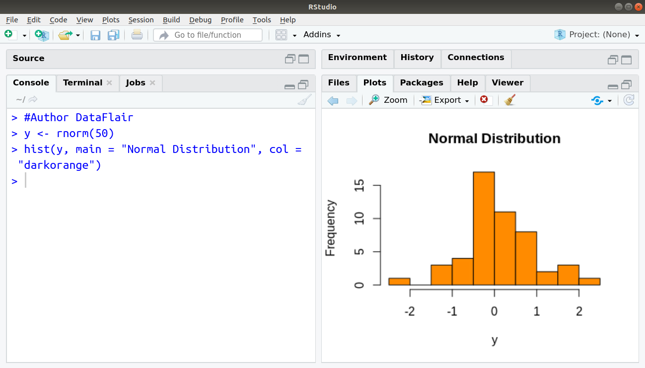
4. rnorm()
Syntax: rnorm(n, mean, sd)
For example:
Create a sample of 50 numbers which are normally distributed.
#Author Dataflair
y <- rnorm(50)
hist(y, main = "Normal Distribution", col = "darkorange")
Output:
Statistical Process Control – A Case Study of Normal Distribution
Statistical Process Control (SPC) was developed at the Bell Labs in the 1920s by Dr Walter Shewhart. The underlying concepts of SPC were implemented in Japanese industries after the end of World War 2. Due to its quality as a tool to improve the product through reduction of process variation, it is being used all around the world.
Reduction of variation is one of the key goals of industries to improve their product quality. There are two main causes that contribute towards the variation – common causes and special causes. With the help of distribution, processes are evaluated based on how centred they are, that is, how close the distribution is towards the mean.
With the help of frequency distributions, control limits with known probabilities are established. Control Limits are useful in minimizing the false alarms, that is, minimizing the probability of finding problems where none exist. A normal distribution is greatly utilized in Statistical Process Control.
Normal Distribution plays a quintessential role in SPC. With the help of normal distributions, the probability of obtaining values beyond the limits is determined. In a Normal Distribution, the probability that a variable will be within +1 or -1 standard deviation of the mean is 0.68. This means that 68% of the values will be within 1 standard deviation of the mean. Furthermore, the probability that the variable will be within 2 of the average will be 0.95 and will have a probability of 0.997 within 3 of the average.
Knowing that 99.7% of the values will fall within 3 standard deviations of the average, it is considered with confidence that value beyond 3 will be highly unlikely. That is if there is no significant change in the process.
Summary
We have studied about normal distribution in R in detail. Moreover, we have learned different functions which are used in generating normal distribution. In the above-mentioned information, we have used graphs, syntax and examples which helps you a lot in an understanding the R normal distribution and their functions.
Now, it’s time for learning Binomial and Poisson Distribution in R Programming
Still, if you have any query regarding normal distribution in R, ask in the comment section.
We work very hard to provide you quality material
Could you take 15 seconds and share your happy experience on Google


it is short so extanded the information
what does these function mean? mere syntax implementattion does not delivery the intended information.
it would be nice if you have mentioned e.g. PNORM what is it? when and where is should be , what o/ps it provide from statistical view, please pt and qt as well . how they help in determining CI and Confidence Inteervals with solved numerical and application . Apart from this Data flair contributig pretty much towards R community by providig beginer the most needed tutorials.
Thanks a ton ………..