Introduction to Contingency Tables in R – A Vital Booster for Mastering R
Expert-led Courses: Transform Your Career – Enroll Now
This R tutorial is all about contingency tables in R. First of all, we will discuss the introduction to R contingency tables and different ways to create contingency tables in R. And, after completing this tutorial, you will thoroughly understand the complex tables/ flat tables, cross tabulation and recreating original data from contingency tables in R.
What are Contingency Tables in R?
A contingency table is particularly useful when a large number of observations need to be condensed into a smaller format whereas a complex (flat) table is a type of contingency table that is used when creating just one single table as opposed to multiple ones.
You can manipulate, alter, and produce table objects using the table() command to summarize a data sample including vector, matrix, list, and data frame objects. You can also create a few special kinds of table objects, like contingency tables and complex (flat) contingency tables using table() command.
Additionally, you can also use cross-tabulation to reassemble data into a tabular format, as required.
Do you know about Object Oriented Programming in R
Making Contingency Tables in R
A contingency table is a way to redraw data and assemble it into a table. And, it shows the layout of the original data in a manner that allows the reader to gain an overall summary of the original data. table() command can be used to create contingency tables in R because the command can handle data in simple vectors or more complex matrix and data frame objects. The more complex the original data, the more complex is the resulting contingency table.
Creating Contingency Tables from Vectors in R
Vector is the simplest data object from which you can create a contingency table. In the following example, you have a simple numeric vector of values.
> #Author DataFlair
> vec = c(3,5,7,9,11,3,6,2,1,9,0,5,4)
> table(vec)
> sort(vec)
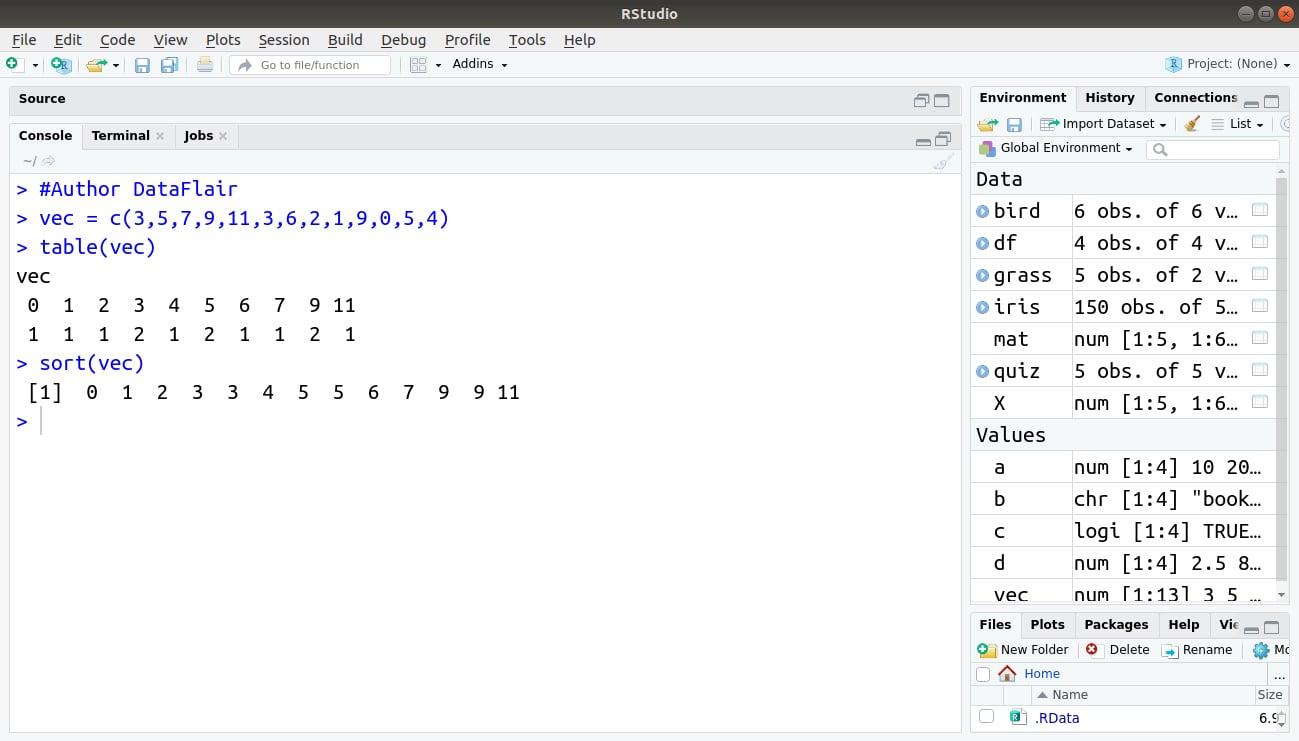
With the help of the sort() command, we are able to obtain a reordered set of data values. We can also compare the sorted values with the output that is obtained when the table() command is applied to it.
Explore the Numeric and Character Functions in R
Creating R Contingency Tables from Data
In this section, we will explain a simple example that provides a data frame containing numeric values in one column and also containing factors in two of its columns. These two columns of factors contain character variables.
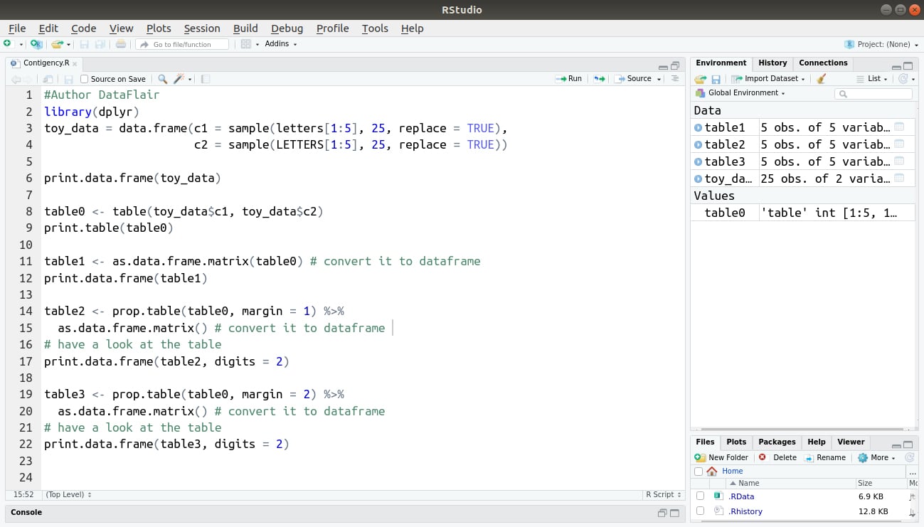
In order to create our contingency table from data, we will make use of the table(), addmargins(), as.data.frame.matrix() and prop.table(). In the following example, the table() function returns a contingency table. Basically, it returns a tabular result of the categorical variables.
#Author DataFlair
library(dplyr)
toy_data = data.frame(c1 = sample(letters[1:5], 25, replace = TRUE),
c2 = sample(LETTERS[1:5], 25, replace = TRUE))
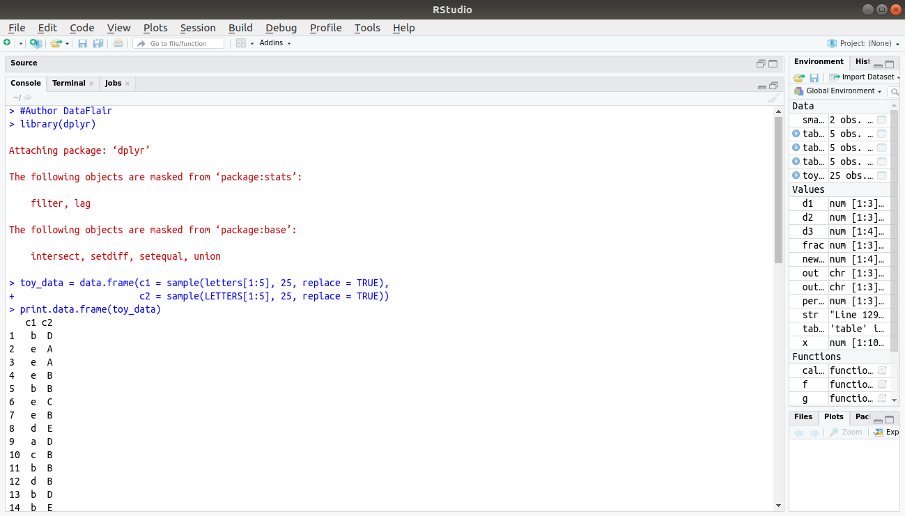
print.data.frame(toy_data)
table0 <- table(toy_data$c1, toy_data$c2)
print.table(table0)
table1 <- as.data.frame.matrix(table0) # convert it to dataframe
print.data.frame(table1)
table2 <- prop.table(table0, margin = 1) %>%
as.data.frame.matrix() # convert it to dataframe
# have a look at the table
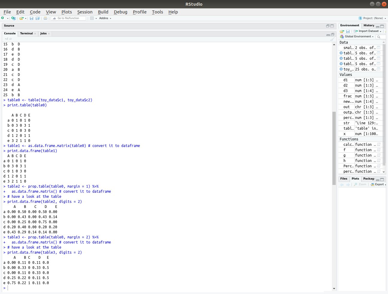
print.data.frame(table2, digits = 2)
table3 <- prop.table(table0, margin = 2) %>%
as.data.frame.matrix() # convert it to dataframe
# have a look at the table
print.data.frame(table3, digits = 2)
We obtain the following output:
How to Create Custom Contingency Tables in R?
The contingency table in R can be created using only a part of the data which is in contrast with collecting data from all the rows and columns. In situations like these, we can perform a selection of each row and column that is to be used.
You can create a custom contingency table in R using the following ways:
- Performing column selection for use in the contingency table.
- Performing selection of the rows that are to be used.
- Carrying out the rotation of data frames.
- Making use of data objects.
- Using data frames.
We will learn about each of these in detail below:
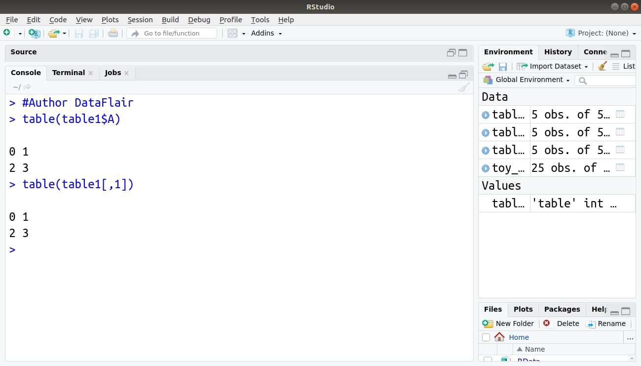
1. Selecting Columns to Use in an R Contingency Table
With the help of table() command, we are able to specify the columns with which the contingency tables can be created. In order to do so, you only need to mention the name of vector objects as follows:
table(table1$A)
This can also be written as:
table(table1[,1])
We obtain the following output when we run these commands in our RStudio:
2. Selecting Rows to Use in R Contingency Table
Rows form the basis of contingency tables. In order to select only certain rows, a different approach is to be adapted. This process requires the creation of an object that is of the matrix form through which you can derive a contingency table using rows that are present in the data frame of the contingency table.
Have you checked – R Data Frame Tutorial
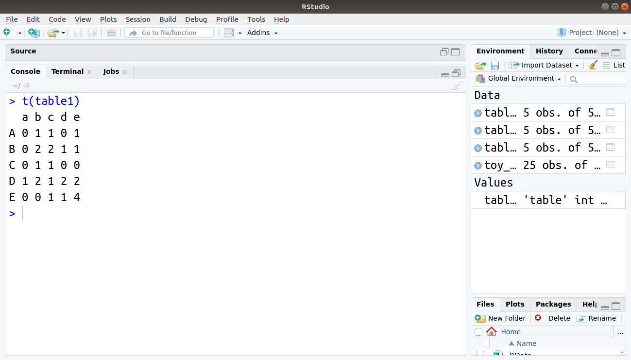
3. Rotating Data Frames in R
You can perform a rotation of the data, that is, transpose of the data using the t() command. This can be carried out as follows:
> t(table1)
We obtain the following output for the transposed table ‘table1’:
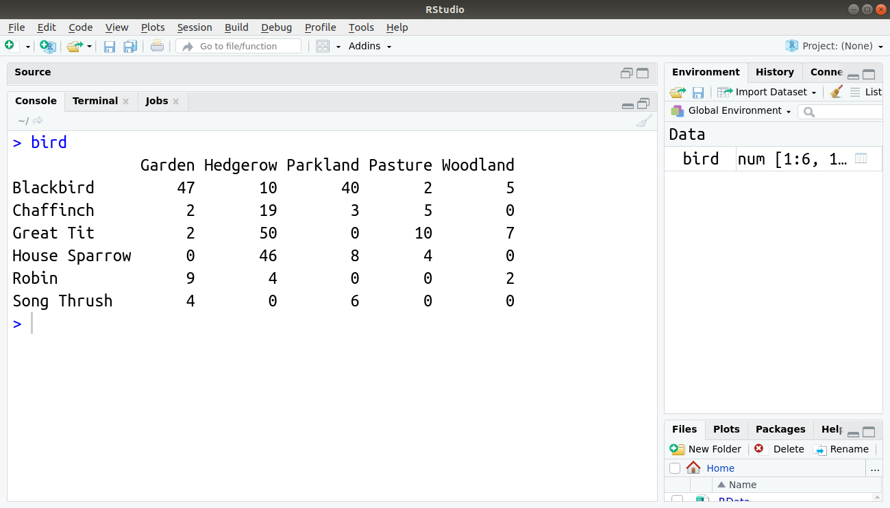
4. Creating Contingency Tables from Matrix Objects in R
For this section, we will create our matrix of bird observation data as follows:
bird = matrix( c(47, 10, 40, 2, 5, 2, 19, 3, 5, 0, 2, 50, 0, 10, 7, 0, 46, 8, 4, 0, 9, 4, 0, 0, 2, 4 ,0, 6, 0,0), nrow=6, ncol=5,byrow = TRUE)                      # fill matrix by rows

dimnames(bird) = list( c("Blackbird", "Chaffinch", "Great Tit",
                      "House Sparrow", "Robin", "Song Thrush"),         # row names
                      c("Garden", "Hedgerow", "Parkland",
                        "Pasture", "Woodland"))                         #Column names
Our matrix “bird” looks like:
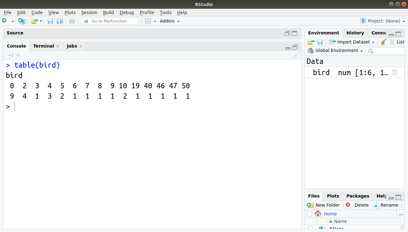
Using the table() command, you will get the result, shown in the following table:
>table(bird)
Understand the R Matrix and Matrix Function in R
5. Using Rows of a Data Frame in a Contingency Table
With the help of this matrix, you can create a contingency table by looking at the rows. However, if there is a data frame, the same cannot be done with the use of bracket convention.
You can get it to work as follows:
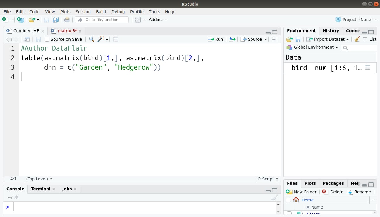
#Author DataFlair
table(as.matrix(bird)[1,], as.matrix(bird)[2,],
      dnn = c("Garden", "Hedgerow"))
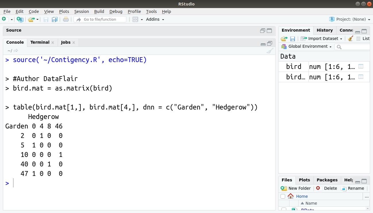
Furthermore, a new matrix can also be created on which the table() command is applied as follows:
#Author DataFlair
bird.mat = as.matrix(bird)
table(bird.mat[1,], bird.mat[4,], dnn = c("Garden", "Hedgerow"))
Selecting Parts of R Table Object
In R, the special type of matrix is a table. Like handling matrix objects, you can also deal with the tables. This also covers extracting matrix objects which are similar to extraction of the table object.
Below some commands are listed for selecting parts of a table object:
> str(pw.tab) – Examines the structure of the table object named tab.
> pw.tab[1:3,] – Displays the first three rows of the contingency table.
> pw.tab[1:3,1] – Displays the first three rows of the first column.
> pw.tab[1:3,1:2] – Displays the first three rows of the first and second columns.
> pw.tab[,’hi’] – Displays the column labeled hi.
> pw.tab[1:3, c(‘hi’, ‘mid’)] – Displays the first three rows of two of the columns.
> pw.tab[1:3, c(‘mid’, ‘hi’)] – Displays some of the columns in a new order.
> pw.tab[,c(‘hi’,3)] – Displays two columns using a mix of name and number.
> length(pw.tab) – Displays the length of the table object.
The first step is to create the table object using two of the columns to produce a simple contingency table. The str() command validates that the resulting object is a table. The table can be displayed much like a matrix by using square brackets to define rows and columns as required. The rows and columns can be specified as numbers or names (if appropriate), but you cannot mix names and numbers in the same command.
The length() command produces a result that reflects the number of items in the table; this is similar to a matrix but different from a data frame (where the command produced a number of columns).
Converting an Object into a Table
As mentioned above, a table is a special type of data object which is similar to the matrix but also possesses several differences.
We make use of the as.table() command for converting an object into a table. This is only valid, however, if the object is in the matrix form. In the case of a data frame, the object can be converted into the matrix and then it can be converted into the table. We will do the same in R as follows:
> as.table(as.matrix(bird))

Testing for R Table Objects
In order to validate if the object is of the table type, we use the is.table() command. The result of this command is Boolean, that is, we will obtain either TRUE or FALSE.
> is.table(bird)

> is.table(table0)
Complex Tables/ Flat Tables in R
Several rows and columns are subdivided to form a single table. This happens in a flat table. We can create the same using an alternative table() command. The ftable() command can be used in various ways such as:
- To construct a “Flat” contingency table in R, we can use the ftable() command.
- You can also make selective “Flat” tables in R.
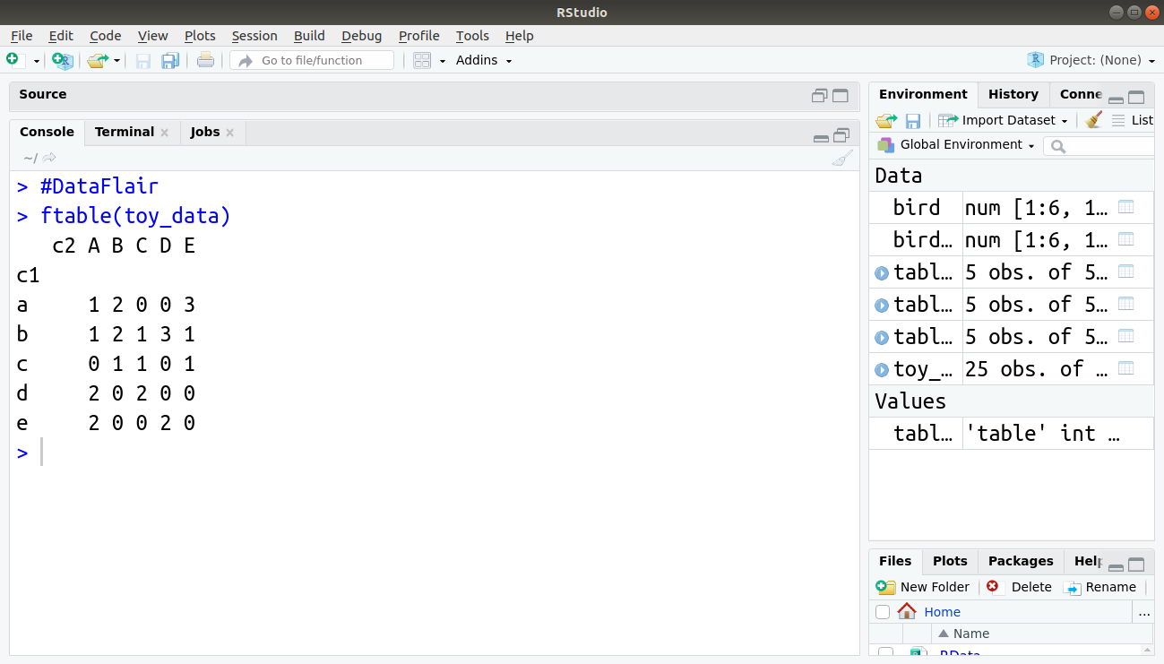
Making “Flat” Contingency Tables in R
The “flat” contingency table in R can be created using the ftable() command as follows:
#DataFlair
ftable(toy_data)
We can also create contingency tables in R with the help of the table() command. We can also specify two or more columns that are to be used in a table. For obtaining a slightly different custom output, we can use a different syntax. The general form of command is: ftable(column.items~row.items, data = data.object)
Wondering what this tilde (~) character means? Well, it is used for creating a formula in places where the left side of the symbol is containing variables in the form of row headings that are separated by the commas. The names of the vectors also form the row items. Before the ~ forms are the column specification whereas to the right, there are groupings of the table in the order of specification.
You must definitely check the Input/ Output Features in R
Testing R Flat Table Objects
For understanding the type of object that is being dealt with, we use the class() command. This command provides a unique label for each kind of the object. With the specification of the class of the object, R is capable of determining the type of object and also specifies the class of it.
The command you can use for testing flat objects is as follows:
if(class(table1) == 'ftable') TRUE else FALSE
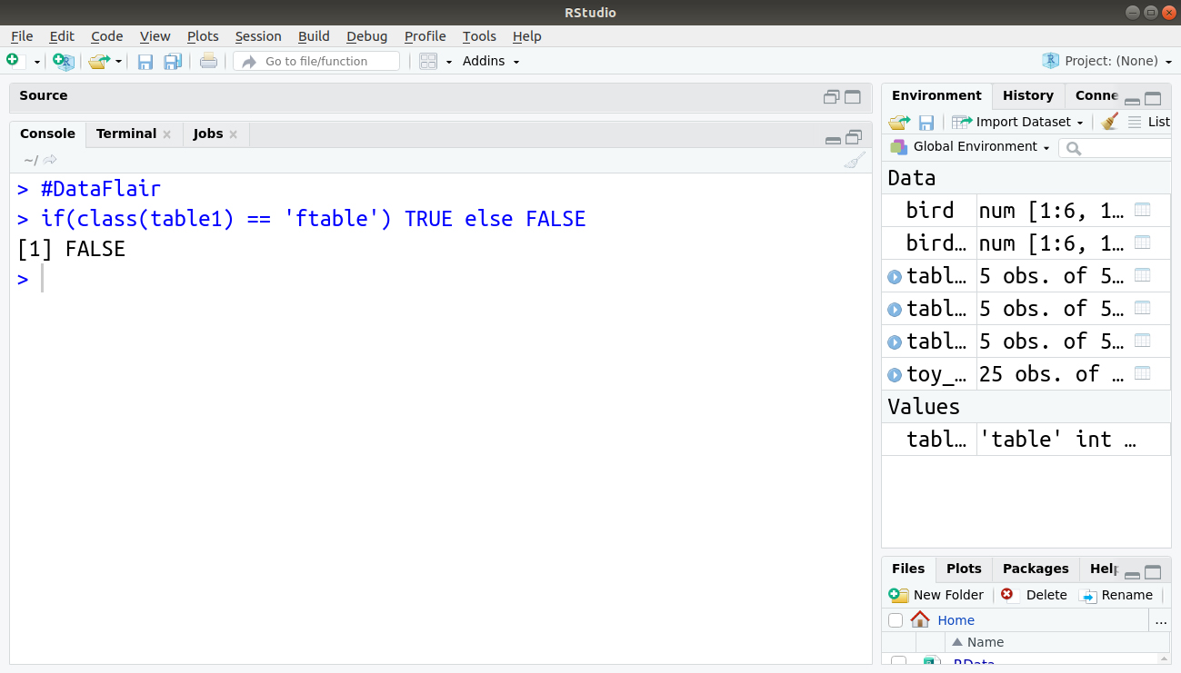
In the above command, the class of the object is not a ‘ftable’ since a FALSE is returned.
R Summary Commands for Tables
A table is a way to summarize data and is often the end point of operation, for example, making a contingency table. However, it is desired to perform certain actions on a table itself.
Some useful summary commands for tables are shown as follows:
- table(x, margin = NULL, FUN) – In order to obtain the various contents of the data frame, matrix or a table, we make use of this command. When specifying margin as 1, we obtain row totals and when the margin is specified as 2, we obtain the column totals.
The prop.table() command is for displaying the proportions of the total sum. The index for rows and columns can also be added through which you can express your data in a better way by various proportions of the rows and column sums. The prop.table() command can be used for displaying contents of the table. This is carried out in proportions of the total sum. Lastly, for expressing the data as proportions of various rows and column sums, you can also add an index.
- addmargin(A, margin = c(1, 2), FUN = sum) – For returning a function that is applied to the rows or columns of a table, we use the addmargin() command. With this command, you can use any function on the rows or columns.
Essentially, you get a row of results. In most situations, you are going to use the function to produce summaries for both rows and columns.
Don’t forget to check the R Recursive Function
Cross Tabulation in R
In order to represent the rows in a tabular format, we make use of the cross tabulation. For doing so, we make use of the xtabs() command as follows:
xtabs(freq.data~categories.list, data)
Notice that the sign tilde (~) is placed on the right-hand side of the frequency of the data.
This is similar to the ftable() command which we discussed above. The logic is the same. That is, towards the left of tilde, we assign the name of the frequency of data and to its right, we assign the categories. These categories can be cross-tabulated with the plus(+) sign.
Finally, we type the name of the data object towards the end and if we don’t, R will not find these variables!
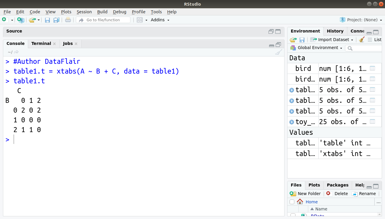
We can use this command on our ‘table1’ data as follows:
> table1.t = xtabs(A ~ B + C, data = table1)
> table1.t
Testing Cross-Table (xtabs) Objects
When you use the xtabs() command, the object you create is a kind of table and gives a TRUE result using the is.table() command. It also gives a TRUE result if you use the as.matrix() command.
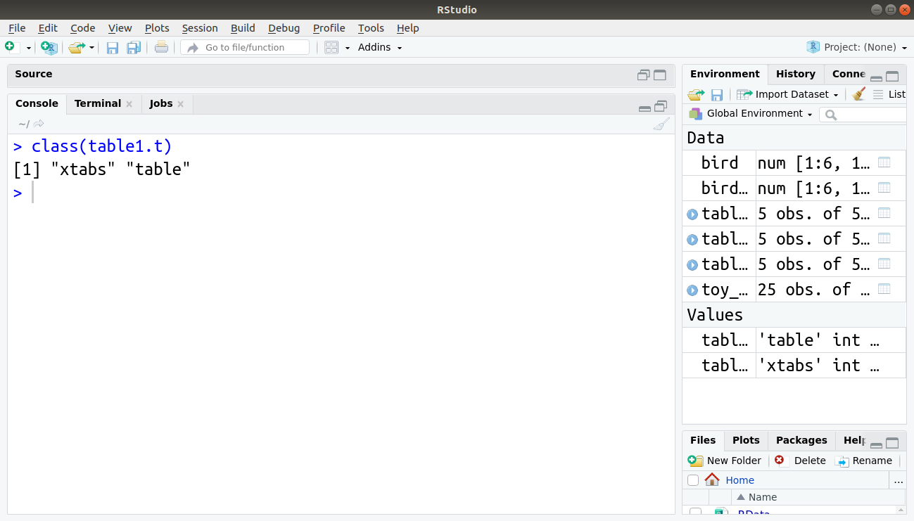
As far as R is concerned, it holds two sorts of class. You can see this using the class() command:
class(table1.t)
If the xtabs object is to be tested, we may face an issue as the class result will possess two elements:
if(class(table1.t) == 'xtabs') TRUE else FALSE
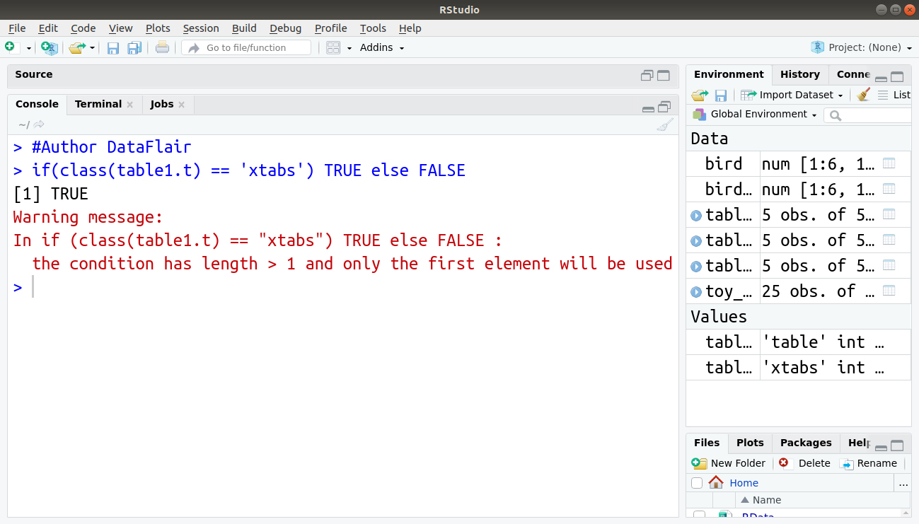
This result is an error message because the ‘xtabs’ result was produced first. There are several refinements to this which are required to pick out the desired values.
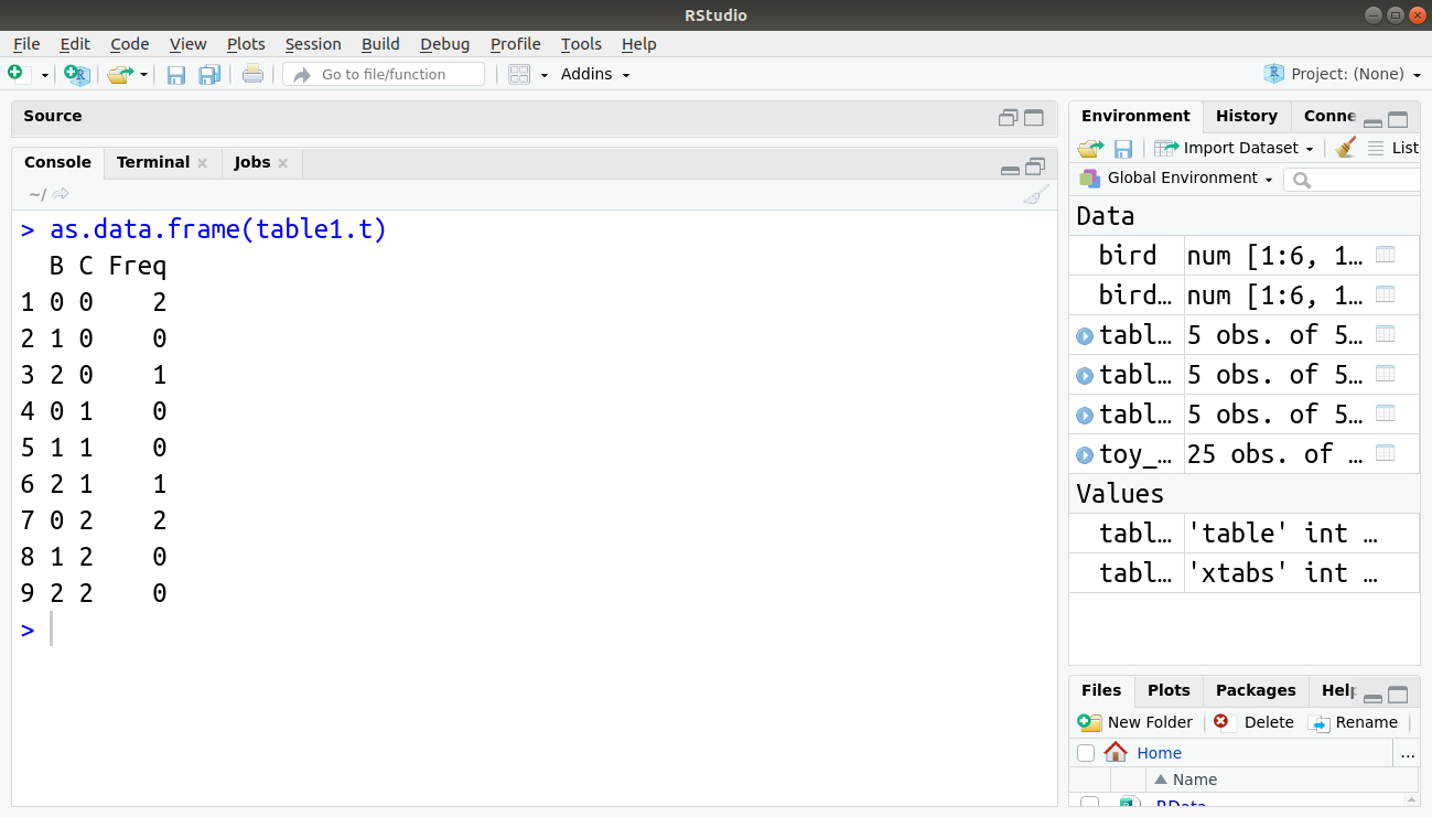
Recreating Original Data from a Contingency Table
The xtabs object can be reassembled into the data frame with the help of as.data.frame() command:
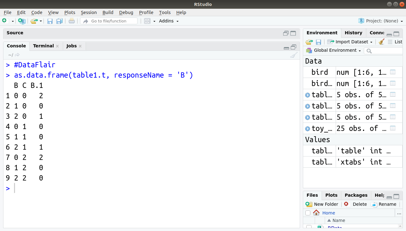
> as.data.frame(table1.t)
as.data.frame(table1.t, responseName = 'B')
Switching Class in R
You can use the class() command to alter the class of an object and see the current class of the object. This can be useful at instances where an object needs to be in a certain class for a command to operate. In the following example, the bird object is queried and then reset using the class() command:
> class(bird)
> attributes(bird)$class <- "table"
> bird
> class(bird)
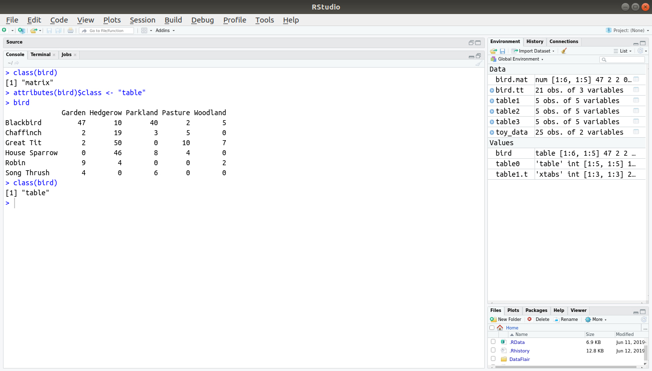
The matrix of bird observations is now classed as a table. You can now proceed to create a data frame from the table using the as.data.frame() command:
> bird.df = as.data.frame(bird)
The columns are not labelled appropriately and the zero data is still intact in the result of the as.data.frame() command. This can be modified by using names() command and reconstruct the data omitting the zero rows, shown as follows:
> bird.tt = bird
> class(bird.tt) = 'table'  #DataFlair
> bird.tt = as.data.frame(bird.tt)
> names(bird.tt) = c('Species', 'Habitat', 'Qty')
> bird.tt = bird.tt[which(bird.tt$Qty > 0),]
> rownames(bird.tt) = as.numeric(1:length(rownames(bird.tt))) #dataflair
> bird.tt
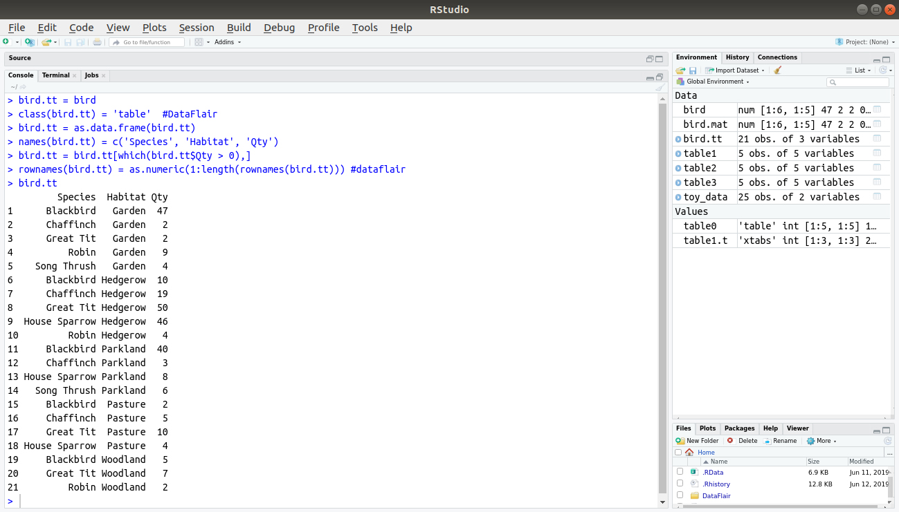
- The first command simply creates a duplicate matrix to work on, keeping the original intact.
- The second command changes the class to “table”.
- The third command creates the data frame of original values.
- The fourth command alters the names of the columns.
- The penultimate command selects out the data that are greater than zero, effectively deleting 0 observations.
- The final command reinstates the row index labels to a continuous sequence.
Summary
In this article, we studied contingency tables in R. This topic is one of the most important concepts and the mastery of it is utmost important to get an in-depth insight into R programming. Furthermore, learning how to manage data by building tables is an important procedure to ensure an efficient process of data analysis. We hope that you enjoyed reading this article.
Next article in your journey of R programming – R Graphical Models Tutorial
If you have any queries or feedback for us, share them in the comment section.
If you are Happy with DataFlair, do not forget to make us happy with your positive feedback on Google


i have two vectors b1 with 3 nonzero values and 7 zeros and b1.est values obtained by running regression which are diffrent in every run . i want to make contingency table i:e
table(b1!=0, b1.est!=0) to compare the non zero values in estimated vector.
table command gives correct results when estimated vector have zero and non zero values, but incorrect results when estimated vector have all zeros or all non zeros. why?????
i want to chek the no of nonzeros which is correctly classified and misclassified.