Machine Learning Project – Data Science Movie Recommendation System Project in R
Expert-led Online Courses: Elevate Your Skills, Get ready for Future - Enroll Now!
Have you ever been on an online streaming platform like Netflix, Amazon Prime, Voot? I watched a movie and after some time, that platform started recommending me different movies and TV shows. I wondered, how the movie streaming platform could suggest me content that appealed to me. Then I came across something known as Recommendation System. This system is capable of learning my watching patterns and providing me with relevant suggestions. Having witnessed the fourth industrial revolution where Artificial Intelligence and other technologies are dominating the market, I am sure that you must have come across a recommendation system in your everyday life. I am also sure that by this time curiosity must be getting the best of you. Therefore, in this Machine Learning Project, I will teach you to build your own Movie recommendation system. So. let’s start.
Movie Recommendation System Project using ML
The main goal of this machine learning project is to build a recommendation engine that recommends movies to users. This R project is designed to help you understand the functioning of how a recommendation system works. We will be developing an Item Based Collaborative Filter. By the end of this tutorial, you will gain experience of implementing your R, Data Science, and Machine learning skills in a real-life project.
Before moving ahead in this movie recommendation system project in ML, you need to know what recommendation system means. Read below to find the answer.
What is a Recommendation System?
A recommendation system provides suggestions to the users through a filtering process that is based on user preferences and browsing history. The information about the user is taken as an input. The information is taken from the input that is in the form of browsing data. This information reflects the prior usage of the product as well as the assigned ratings.
A recommendation system is a platform that provides its users with various contents based on their preferences and likings. A recommendation system takes the information about the user as an input. The recommendation system is an implementation of the machine learning algorithms.
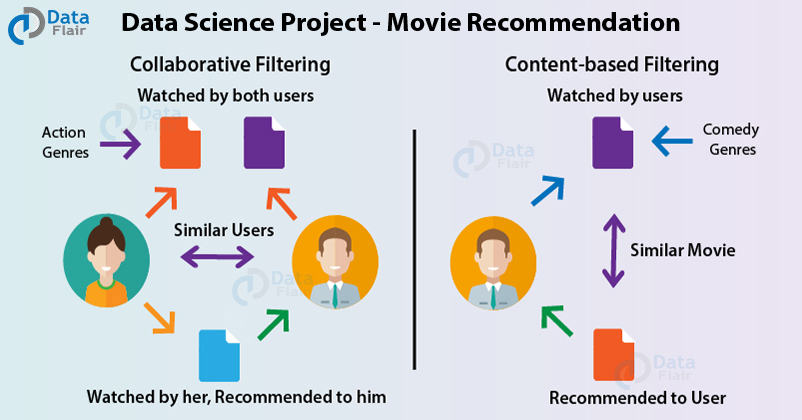
A recommendation system also finds a similarity between the different products. For example, Netflix Recommendation System provides you with the recommendations of the movies that are similar to the ones that have been watched in the past. Furthermore, there is a collaborative content filtering that provides you with the recommendations in respect with the other users who might have a similar viewing history or preferences.
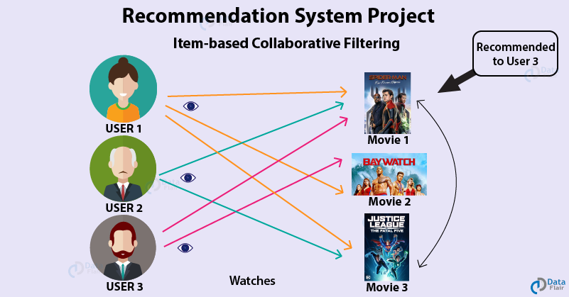
There are two types of recommendation systems – Content-Based Recommendation System and Collaborative Filtering Recommendation. In this project of recommendation system in R, we will work on a collaborative filtering recommendation system and more specifically, ITEM based collaborative recommendation system.
The biggest benefit of the collaborative filtering approach and especially the item-based one is that it can benefit from the interaction between users and items, thus, while recommending items, it can search for patterns in grouping of the items. Thus, this method does not involve comprehending the content of the items, and, therefore, it can be applied to any type of products and services. Also, it is capable of analyzing big data, and the users get their recommendations in real-time.
You must check how Netflix recommendation engine works
How to build a Movie Recommendation System using Machine Learning
Dataset
In order to build our recommendation system, we have used the MovieLens Dataset. You can find the movies.csv and ratings.csv file that we have used in our Recommendation System Project here. This data consists of 105339 ratings applied over 10329 movies.
Importing Essential Libraries
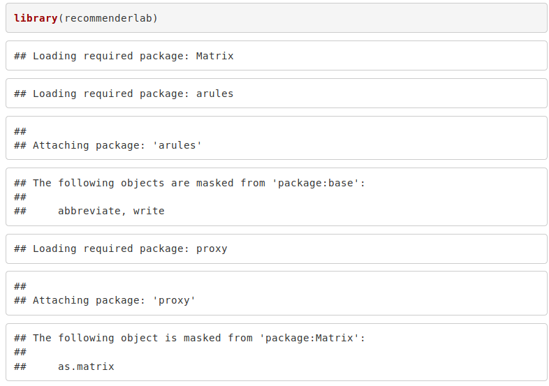
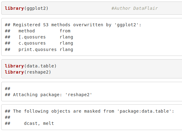
In our Data Science project, we will make use of these four packages – ‘recommenderlab’, ‘ggplot2’, ‘data.table’ and ‘reshape2’.
Code:
library(recommenderlab)
Output Screenshot:
Code:
library(ggplot2)                       #Author DataFlair
library(data.table)
library(reshape2)
Output Screenshot:
Wait! Don’t forget to check our leading guide on R programming classification
Retrieving the Data
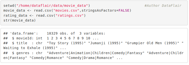
We will now retrieve our data from movies.csv into movie_data dataframe and ratings.csv into rating_data. We will use the str() function to display information about the movie_data dataframe.
Code:
setwd("/home/dataflair/data/movie_data")                       #Author DataFlair
movie_data <- read.csv("movies.csv",stringsAsFactors=FALSE)
rating_data <- read.csv("ratings.csv")
str(movie_data)
Output Screenshot:
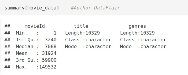
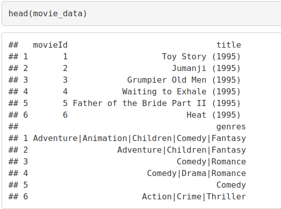
We can overview the summary of the movies using the summary() function. We will also use the head() function to print the first six lines of movie_data
Code:
summary(movie_data) #Author DataFlair
Output Screenshot:
Code:
head(movie_data)
Output Screenshot:
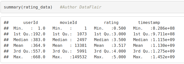
Similarly, we can output the summary as well as the first six lines of the ‘rating_data’ dataframe –
Code:
summary(rating_data) #Author DataFlair
Output Screenshot:
Code:
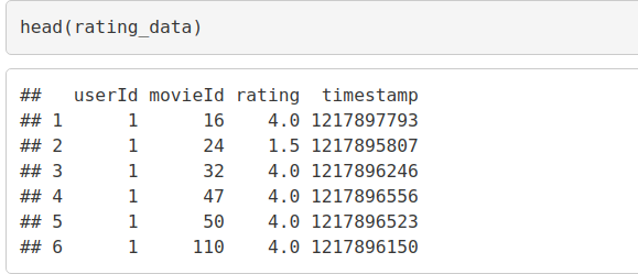
head(rating_data)
Output Screenshot:
Revise your R concepts with DataFlair for Free, checkout 120+ FREE R Tutorials
Data Pre-processing
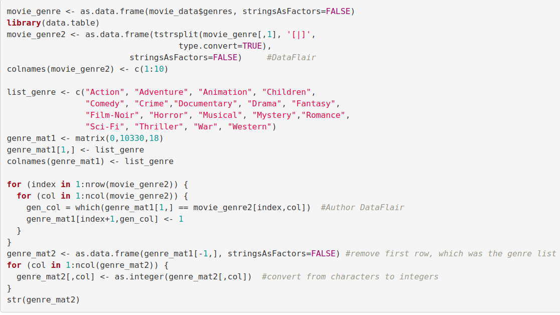
From the above table, we observe that the userId column, as well as the movieId column, consist of integers. Furthermore, we need to convert the genres present in the movie_data dataframe into a more usable format by the users. In order to do so, we will first create a one-hot encoding to create a matrix that comprises of corresponding genres for each of the films.
Code:
movie_genre <- as.data.frame(movie_data$genres, stringsAsFactors=FALSE)
library(data.table)
movie_genre2 <- as.data.frame(tstrsplit(movie_genre[,1], '[|]',
type.convert=TRUE),
stringsAsFactors=FALSE) #DataFlair
colnames(movie_genre2) <- c(1:10)
list_genre <- c("Action", "Adventure", "Animation", "Children",
"Comedy", "Crime","Documentary", "Drama", "Fantasy",
"Film-Noir", "Horror", "Musical", "Mystery","Romance",
"Sci-Fi", "Thriller", "War", "Western")
genre_mat1 <- matrix(0,10330,18)
genre_mat1[1,] <- list_genre
colnames(genre_mat1) <- list_genre
for (index in 1:nrow(movie_genre2)) {
for (col in 1:ncol(movie_genre2)) {
gen_col = which(genre_mat1[1,] == movie_genre2[index,col]) #Author DataFlair
genre_mat1[index+1,gen_col] <- 1
}
}
genre_mat2 <- as.data.frame(genre_mat1[-1,], stringsAsFactors=FALSE) #remove first row, which was the genre list
for (col in 1:ncol(genre_mat2)) {
genre_mat2[,col] <- as.integer(genre_mat2[,col]) #convert from characters to integers
}
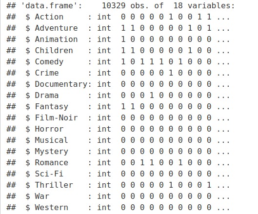
str(genre_mat2)Screenshot:
Output –
In the next step of Data Pre-processing of R project, we will create a ‘search matrix’ that will allow us to perform an easy search of the films by specifying the genre present in our list.
Code:
SearchMatrix <- cbind(movie_data[,1:2], genre_mat2[])
head(SearchMatrix)    #DataFlair
Output Screenshot:
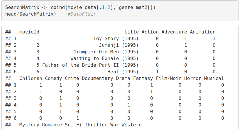
There are movies that have several genres, for example, Toy Story, which is an animated film also falls under the genres of Comedy, Fantasy, and Children. This applies to the majority of the films.
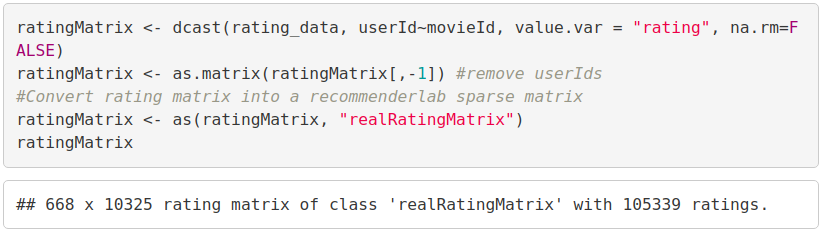
For our movie recommendation system to make sense of our ratings through recommenderlabs, we have to convert our matrix into a sparse matrix one. This new matrix is of the class ‘realRatingMatrix’. This is performed as follows:
Code:
ratingMatrix <- dcast(rating_data, userId~movieId, value.var = "rating", na.rm=FALSE)
ratingMatrix <- as.matrix(ratingMatrix[,-1]) #remove userIds
#Convert rating matrix into a recommenderlab sparse matrix
ratingMatrix <- as(ratingMatrix, "realRatingMatrix")
ratingMatrix
Output Screenshot:
Are you facing any trouble in implementing recommendation system project in R? Comment below, DataFlair Team is ready to help you.
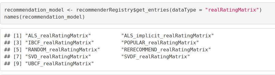
Let us now overview some of the important parameters that provide us various options for building recommendation systems for movies-
Code:
recommendation_model <- recommenderRegistry$get_entries(dataType = "realRatingMatrix")
names(recommendation_model)
Output Screenshot:
Code:
lapply(recommendation_model, "[[", "description")
Output Screenshot:

Want to become the next data scientist? Try out the best way and explore Data Science Tutorials Series to learn Data Science in an easy way with DataFlair!!
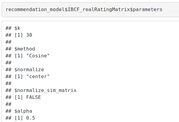
We will implement a single model in our R project – Item Based Collaborative Filtering.
Code:
recommendation_model$IBCF_realRatingMatrix$parameters
Output Screenshot:
Exploring Similar Data
Collaborative Filtering involves suggesting movies to the users that are based on collecting preferences from many other users. For example, if a user A likes to watch action films and so does user B, then the movies that the user B will watch in the future will be recommended to A and vice-versa. Therefore, recommending movies is dependent on creating a relationship of similarity between the two users. With the help of recommenderlab, we can compute similarities using various operators like cosine, pearson as well as jaccard.
Code:
similarity_mat <- similarity(ratingMatrix[1:4, ],
                               method = "cosine",
                               which = "users")
as.matrix(similarity_mat)

image(as.matrix(similarity_mat), main = "User's Similarities")
Output Screenshot:
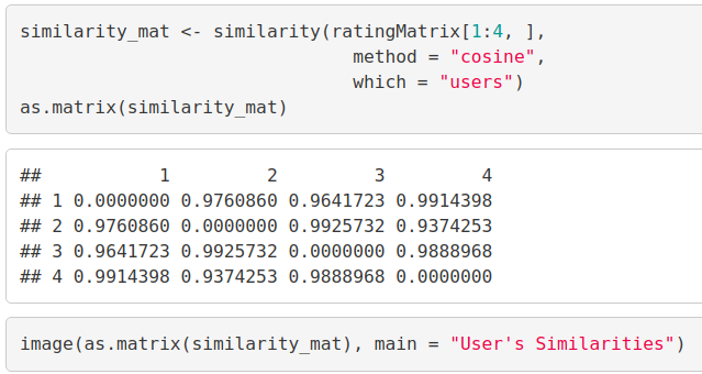
In the above matrix, each row and column represents a user. We have taken four users and each cell in this matrix represents the similarity that is shared between the two users.
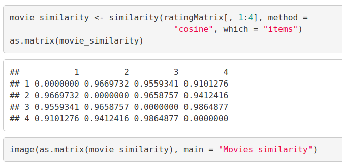
Now, we delineate the similarity that is shared between the films –
Code:
movie_similarity <- similarity(ratingMatrix[, 1:4], method =
                                 "cosine", which = "items")
as.matrix(movie_similarity)

image(as.matrix(movie_similarity), main = "Movies similarity")
Output Screenshot:
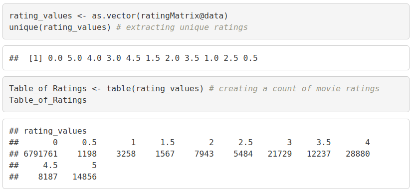
Let us now extract the most unique ratings –
rating_values <- as.vector(ratingMatrix@data)
unique(rating_values) # extracting unique ratings
Now, we will create a table of ratings that will display the most unique ratings.
Code:
Table_of_Ratings <- table(rating_values) # creating a count of movie ratings
Table_of_Ratings
Output Screenshot:
This is the right time to check your R and Data Science Learning. Try these latest interview questions and become a pro.
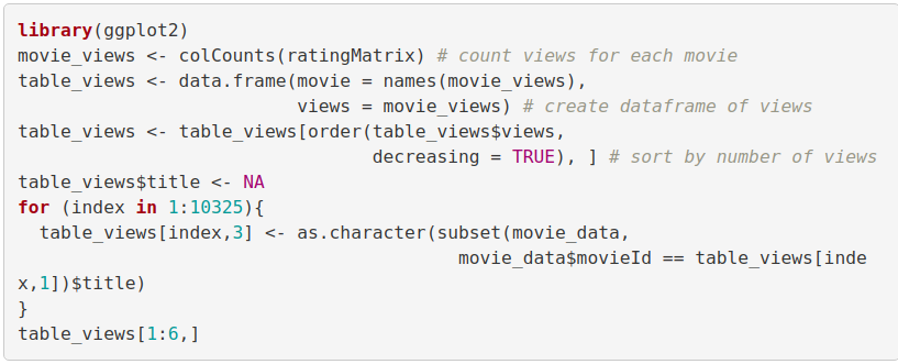
Most Viewed Movies Visualization
In this section of the machine learning project, we will explore the most viewed movies in our dataset. We will first count the number of views in a film and then organize them in a table that would group them in descending order.
Code:
library(ggplot2)
movie_views <- colCounts(ratingMatrix) # count views for each movie
table_views <- data.frame(movie = names(movie_views),
views = movie_views) # create dataframe of views
table_views <- table_views[order(table_views$views,
decreasing = TRUE), ] # sort by number of views
table_views$title <- NA
for (index in 1:10325){
table_views[index,3] <- as.character(subset(movie_data,
movie_data$movieId == table_views[index,1])$title)
}
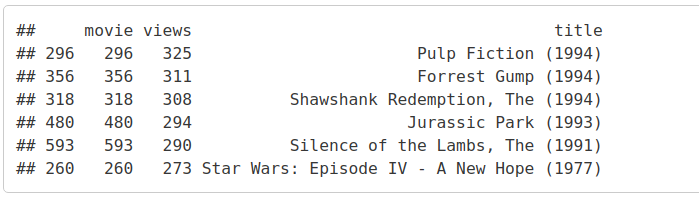
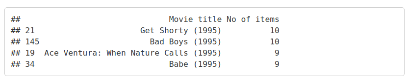
table_views[1:6,]Input Screenshot:
Output –
Now, we will visualize a bar plot for the total number of views of the top films. We will carry this out using ggplot2.
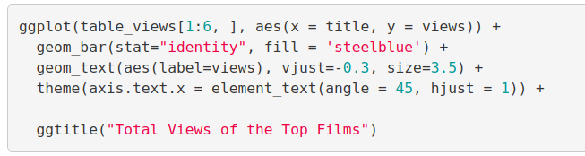
Code:
ggplot(table_views[1:6, ], aes(x = title, y = views)) +
  geom_bar(stat="identity", fill = 'steelblue') +
  geom_text(aes(label=views), vjust=-0.3, size=3.5) +
  theme(axis.text.x = element_text(angle = 45, hjust = 1)) +

  ggtitle("Total Views of the Top Films")
Input Screenshot:
Output:
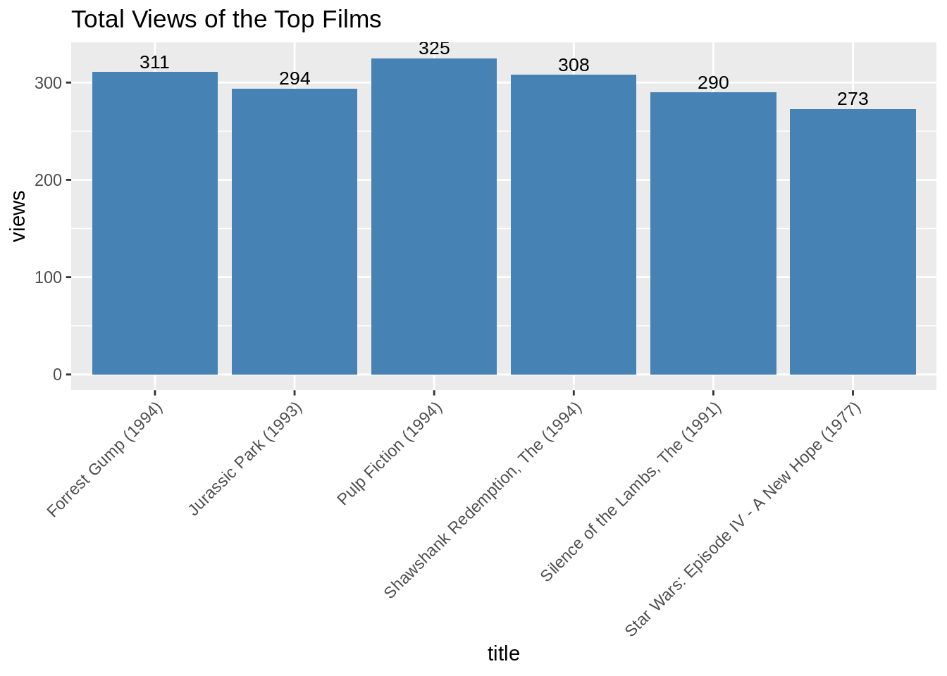
From the above bar-plot, we observe that Pulp Fiction is the most-watched film followed by Forrest Gump.
If you are enjoying this Data Science Recommendation System Project, DataFlair brings another project for you – Credit Card Fraud Detection using R. Save the link, you can thank me later😉
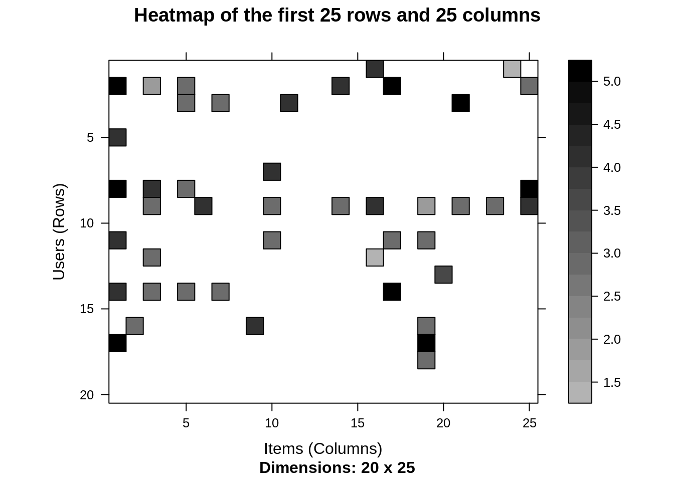
Heatmap of Movie Ratings
Now, in this data science project of Recommendation system, we will visualize a heatmap of the movie ratings. This heatmap will contain first 25 rows and 25 columns as follows –
Code:
image(ratingMatrix[1:20, 1:25], axes = FALSE, main = "Heatmap of the first 25 rows and 25 columns")
Input Screenshot:

Output:
Performing Data Preparation
We will conduct data preparation in the following three steps –
- Selecting useful data.
- Normalizing data.
- Binarizing the data.
For finding useful data in our dataset, we have set the threshold for the minimum number of users who have rated a film as 50. This is also same for minimum number of views that are per film. This way, we have filtered a list of watched films from least-watched ones.
Code:
movie_ratings <- ratingMatrix[rowCounts(ratingMatrix) > 50,
                             colCounts(ratingMatrix) > 50]
Movie_ratings
Output Screenshot:
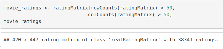
From the above output of ‘movie_ratings’, we observe that there are 420 users and 447 films as opposed to the previous 668 users and 10325 films. We can now delineate our matrix of relevant users as follows –
Code:
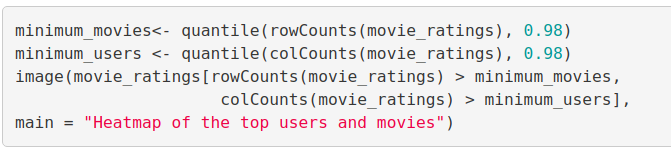
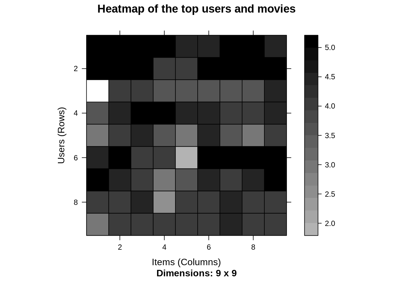
minimum_movies<- quantile(rowCounts(movie_ratings), 0.98)
minimum_users <- quantile(colCounts(movie_ratings), 0.98)
image(movie_ratings[rowCounts(movie_ratings) > minimum_movies,
                     colCounts(movie_ratings) > minimum_users],
main = "Heatmap of the top users and movies")
Input Screenshot:
Output:
Data Visualization in R – Learn the concepts in an easy way
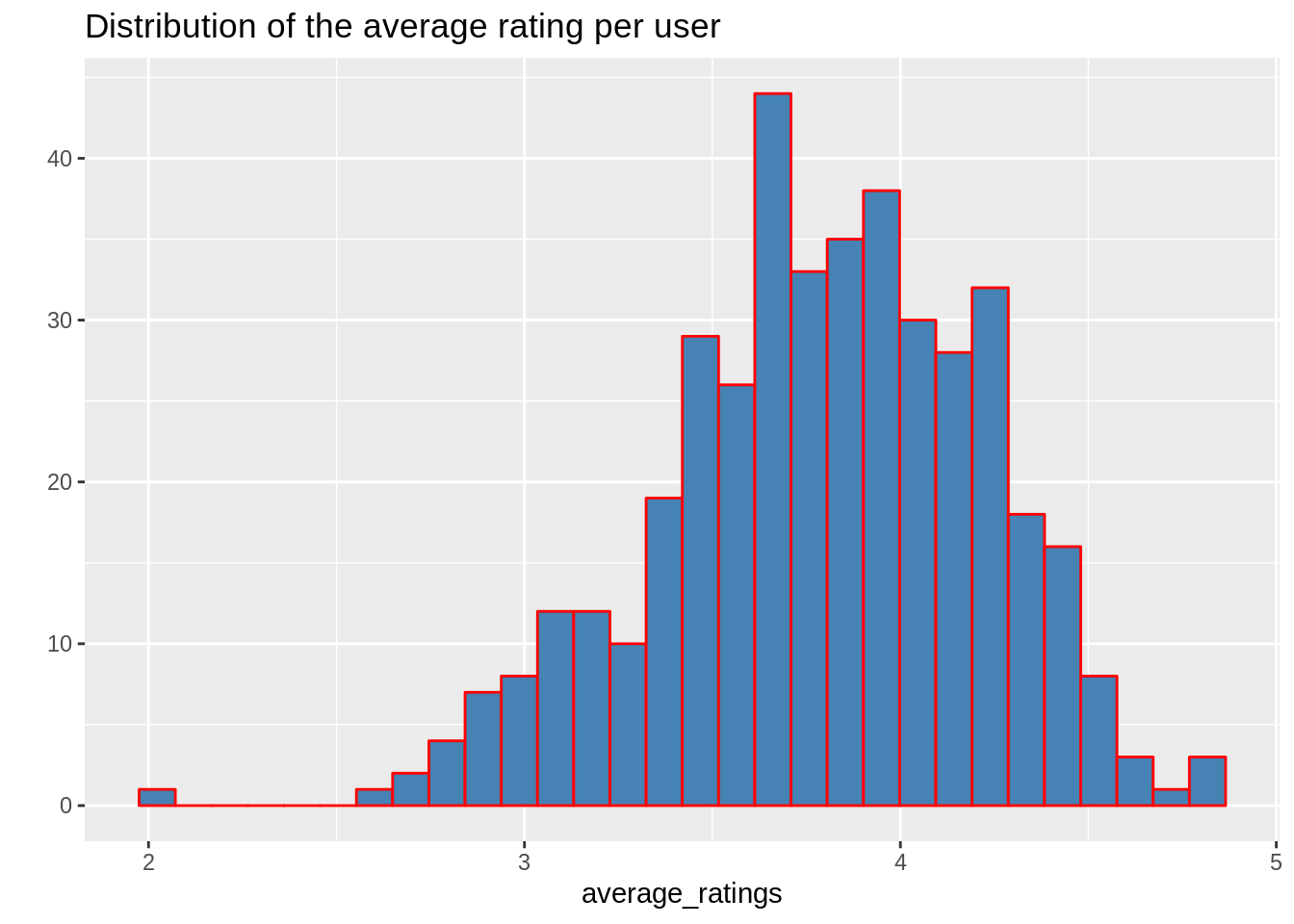
Now, we will visualize the distribution of the average ratings per user.
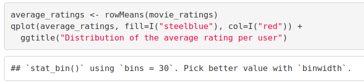
average_ratings <- rowMeans(movie_ratings)
qplot(average_ratings, fill=I("steelblue"), col=I("red")) +
  ggtitle("Distribution of the average rating per user")
Output Screenshot:
Output:
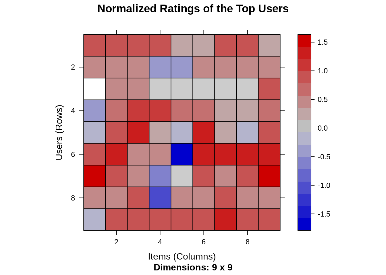
Data Normalization
In the case of some users, there can be high ratings or low ratings provided to all of the watched films. This will act as a bias while implementing our model. In order to remove this, we normalize our data. Normalization is a data preparation procedure to standardize the numerical values in a column to a common scale value. This is done in such a way that there is no distortion in the range of values. Normalization transforms the average value of our ratings column to 0. We then plot a heatmap that delineates our normalized ratings.
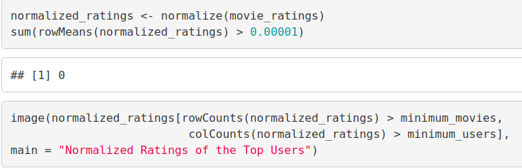
Code:
normalized_ratings <- normalize(movie_ratings)
sum(rowMeans(normalized_ratings) > 0.00001)

image(normalized_ratings[rowCounts(normalized_ratings) > minimum_movies,
                          colCounts(normalized_ratings) > minimum_users],
main = "Normalized Ratings of the Top Users")
Output Screenshot:
Output:
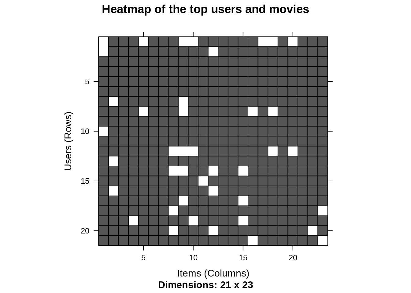
Performing Data Binarization
In the final step of our data preparation in this data science project, we will binarize our data. Binarizing the data means that we have two discrete values 1 and 0, which will allow our recommendation systems to work more efficiently. We will define a matrix that will consist of 1 if the rating is above 3 and otherwise it will be 0.
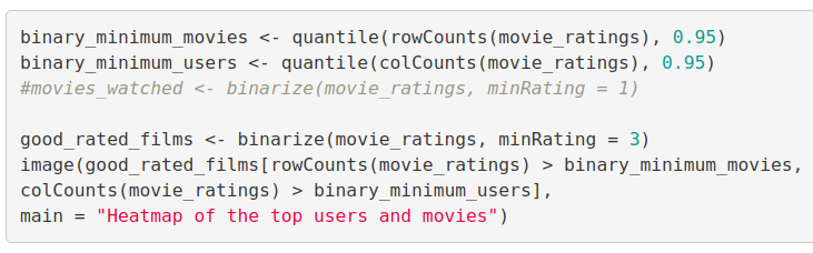
Code:
binary_minimum_movies <- quantile(rowCounts(movie_ratings), 0.95)
binary_minimum_users <- quantile(colCounts(movie_ratings), 0.95)
#movies_watched <- binarize(movie_ratings, minRating = 1)

good_rated_films <- binarize(movie_ratings, minRating = 3)
image(good_rated_films[rowCounts(movie_ratings) > binary_minimum_movies,
colCounts(movie_ratings) > binary_minimum_users],
main = "Heatmap of the top users and movies")
Input Screenshot:
Output:
Didn’t you check what’s trending on DataFlair? Check out the latest Machine Learning Tutorial Series. Master all the ML concepts for FREE NOW!!
Collaborative Filtering System
In this section of data science project, we will develop our very own Item Based Collaborative Filtering System. This type of collaborative filtering finds similarity in the items based on the people’s ratings of them. The algorithm first builds a similar-items table of the customers who have purchased them into a combination of similar items. This is then fed into the recommendation system.
The similarity between single products and related products can be determined with the following algorithm –
- For each Item i1 present in the product catalog, purchased by customer C.
- And, for each item i2 also purchased by the customer C.
- Create record that the customer purchased items i1 and i2.
- Calculate the similarity between i1 and i2.
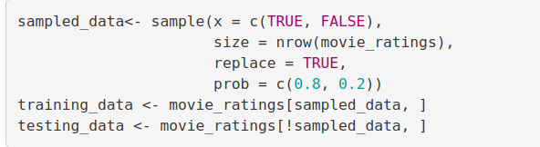
We will build this filtering system by splitting the dataset into 80% training set and 20% test set.
Code:
sampled_data<- sample(x = c(TRUE, FALSE),
                      size = nrow(movie_ratings),
                      replace = TRUE,
                      prob = c(0.8, 0.2))
training_data <- movie_ratings[sampled_data, ]
testing_data <- movie_ratings[!sampled_data, ]
Input Screenshot:
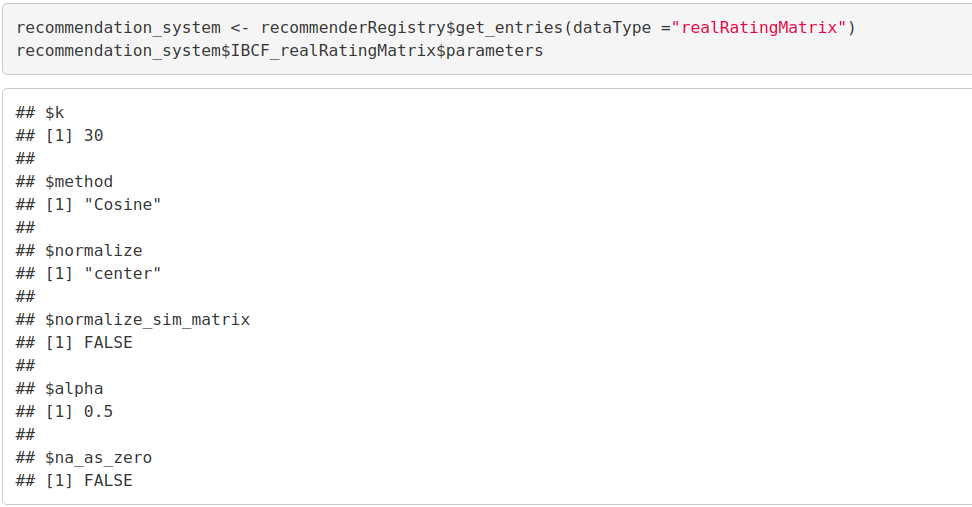
Building the Recommendation System using R
We will now explore the various parameters of our Item Based Collaborative Filter. These parameters are default in nature. In the first step, k denotes the number of items for computing their similarities. Here, k is equal to 30. Therefore, the algorithm will now identify the k most similar items and store their number. We use the cosine method which is the default one but you can also use pearson method.
Code:
recommendation_system <- recommenderRegistry$get_entries(dataType ="realRatingMatrix")
recommendation_system$IBCF_realRatingMatrix$parameters
Output Screenshot:
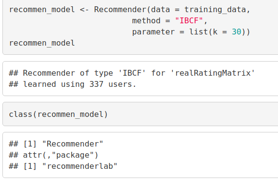
Code:
recommen_model <- Recommender(data = training_data,
                          method = "IBCF",
                          parameter = list(k = 30))
recommen_model
class(recommen_model)
Output Screenshot:
Let us now explore our data science recommendation system model as follows –
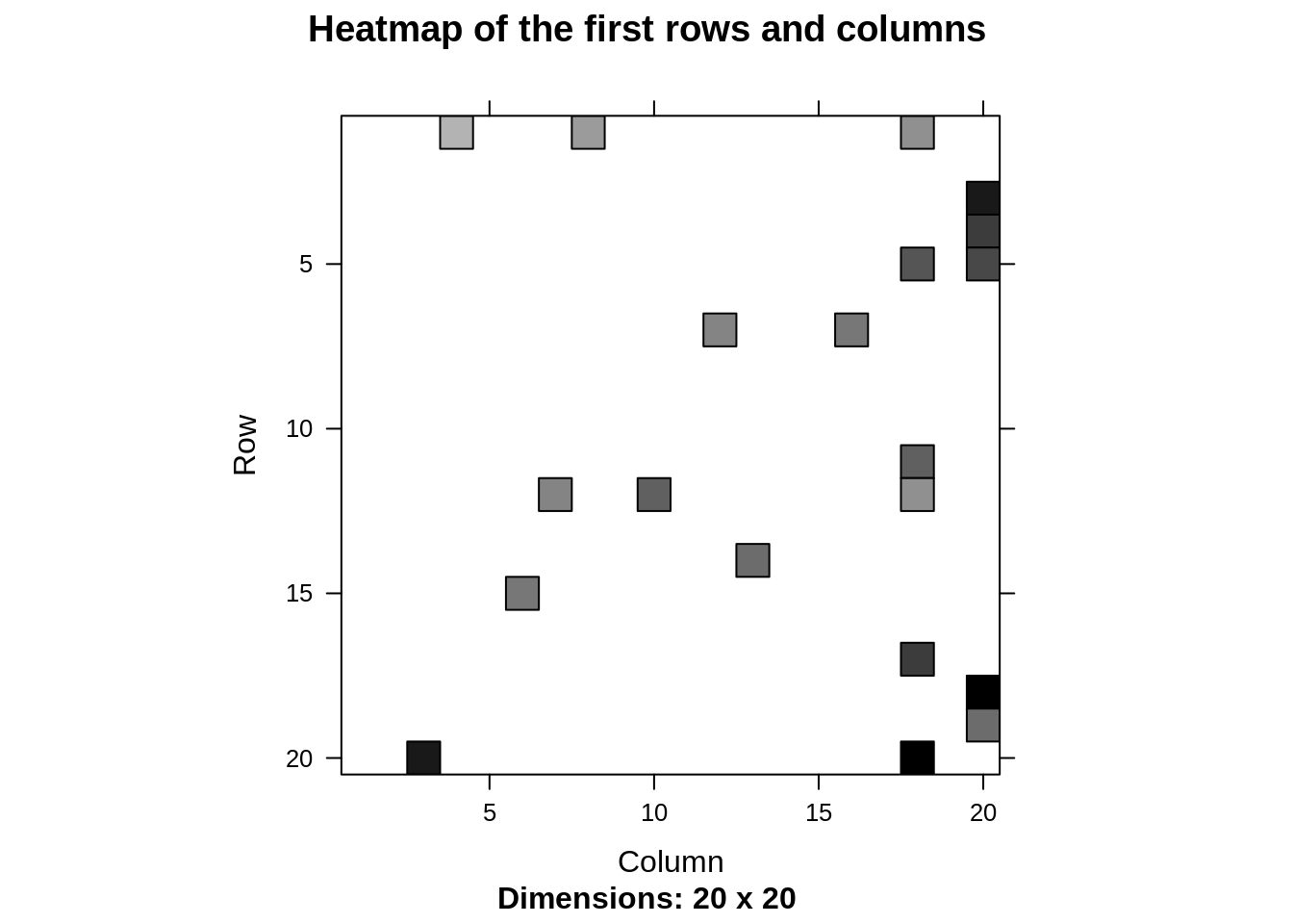
Using the getModel() function, we will retrieve the recommen_model. We will then find the class and dimensions of our similarity matrix that is contained within model_info. Finally, we will generate a heatmap, that will contain the top 20 items and visualize the similarity shared between them.
Code:
model_info <- getModel(recommen_model)
class(model_info$sim)
dim(model_info$sim)
top_items <- 20
image(model_info$sim[1:top_items, 1:top_items],
   main = "Heatmap of the first rows and columns")
Output Screenshot:
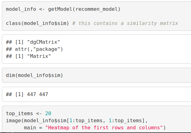
Output:
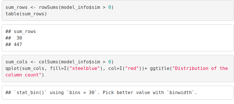
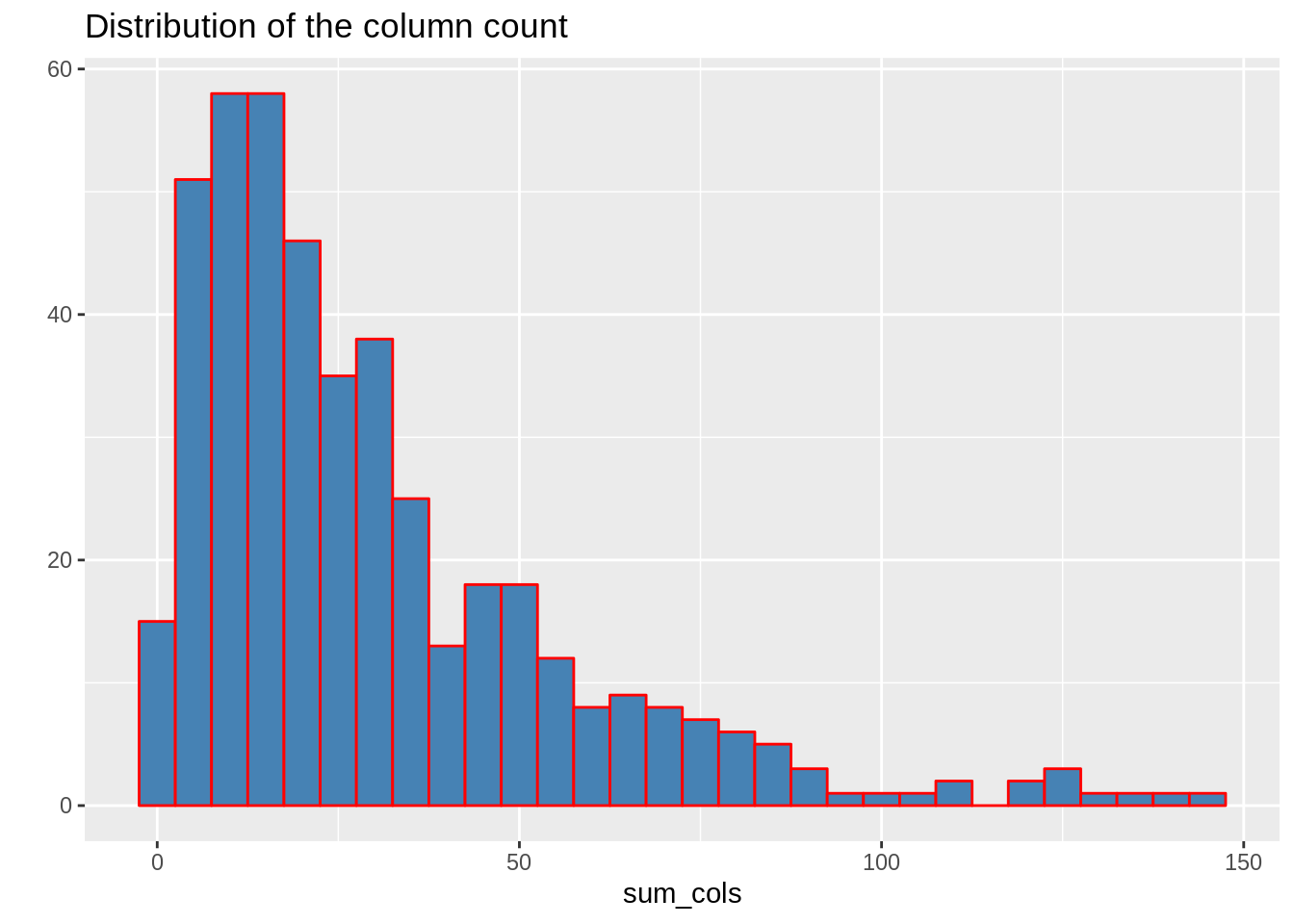
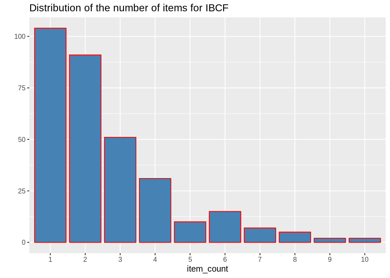
In the next step of ML project, we will carry out the sum of rows and columns with the similarity of the objects above 0. We will visualize the sum of columns through a distribution as follows –
Code:
sum_rows <- rowSums(model_info$sim > 0)
table(sum_rows)

sum_cols <- colSums(model_info$sim > 0)
qplot(sum_cols, fill=I("steelblue"), col=I("red"))+ ggtitle("Distribution of the column count")
Output Screenshot:
Output:
How to build Recommender System on dataset using R?
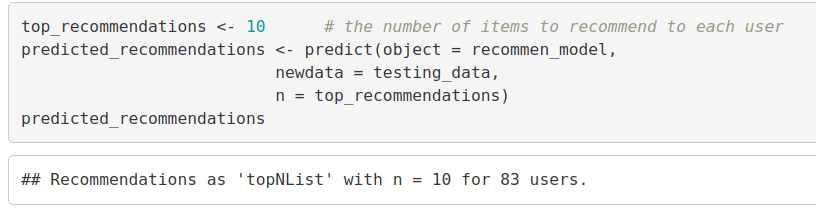
We will create a top_recommendations variable which will be initialized to 10, specifying the number of films to each user. We will then use the predict() function that will identify similar items and will rank them appropriately. Here, each rating is used as a weight. Each weight is multiplied with related similarities. Finally, everything is added in the end.
Code:
top_recommendations <- 10 # the number of items to recommend to each user
predicted_recommendations <- predict(object = recommen_model,
                          newdata = testing_data,
                          n = top_recommendations)
predicted_recommendations
Output Screenshot:
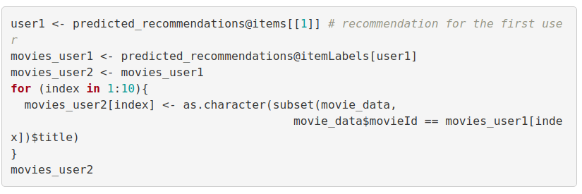
Code:
user1 <- predicted_recommendations@items[[1]] # recommendation for the first user
movies_user1 <- predicted_recommendations@itemLabels[user1]
movies_user2 <- movies_user1
for (index in 1:10){
movies_user2[index] <- as.character(subset(movie_data,
movie_data$movieId == movies_user1[index])$title)
}
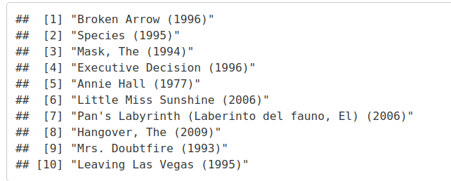
movies_user2Output Screenshot:
Output:
Code:
recommendation_matrix <- sapply(predicted_recommendations@items,
                      function(x){ as.integer(colnames(movie_ratings)[x]) }) # matrix with the recommendations for each user
#dim(recc_matrix)
recommendation_matrix[,1:4]
Output Screenshot:
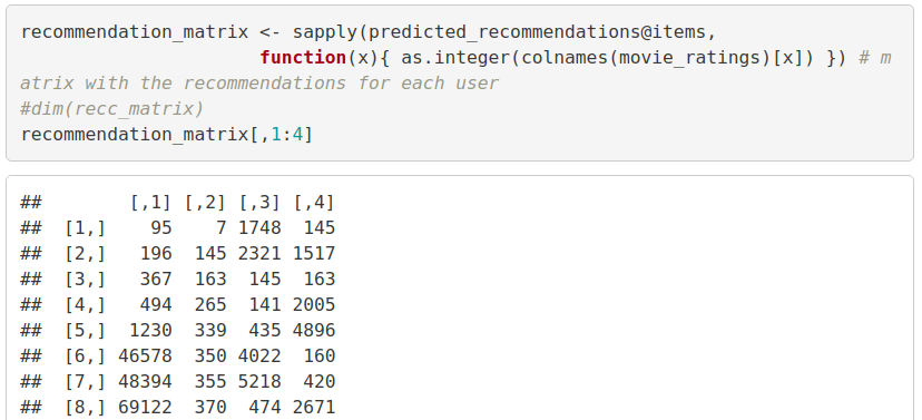
Output:
Summary
Recommendation Systems are the most popular type of machine learning applications that are used in all sectors. They are an improvement over the traditional classification algorithms as they can take many classes of input and provide similarity ranking based algorithms to provide the user with accurate results. These recommendation systems have evolved over time and have incorporated many advanced machine learning techniques to provide the users with the content that they want.
Hola!! You completed this amazing Data Science Recommendation System Project. What next? Another project? Check Sentiment Analysis project in R
Did you enjoy this R project? Have you built any Recommendation System in the past? Do share your experiences in the comments below.
If you are Happy with DataFlair, do not forget to make us happy with your positive feedback on Google


Hello. When i create ratingMatrix i get error “cannot allocate vector of size 113.7 Gb”. ratingMatrix <- dcast(rating_data, userId~movieId, value.var = "rating", na.rm=FALSE)
How to avoid it or what to do to continue working?
Hi, while running the code I have received multiple errors.
1. While running the for loop, I am getting an error as stated below
for (index in 1:nrow(movie_genre2)) {
+ for (col in 1:ncol(movie_genre2)) {
+ gen_col = which(genre_mat1[1,] == movie_genre2[index,col])
+ genre_mat1[index+1,gen_col] <- 1
+ }
+ }
Error in `[ SearchMatrix head(SearchMatrix)
Error in h(simpleError(msg, call)) :
error in evaluating the argument ‘x’ in selecting a method for function ‘head’: object ‘SearchMatrix’ not found
What is the point of the heatmaps for normalization, binarization (under section Performing Data Preparation) when they aren’t actually used in the recommendation system?
I need help can somebody give me email please
when i try to do the searchmatrix < cbind i get the error below
SearchMatrix <- cbind(movie_data[,1:2], genre_mat2[])
Error in data.frame(…, check.names = FALSE) :
arguments imply differing number of rows: 27278, 10329
It’s very usefull
In the following line isn’t it 20 rows and 25 columns
image(ratingMatrix[1:20, 1:25], axes = FALSE, main = “Heatmap of the first 25 rows and 25 columns”)
There is no code associated with the last two outputs
Where is the code to get the last bar chart?
can we get the source code in python?