Introduction to Bayesian Methods – Understand all the Methods thoroughly!
FREE Online Courses: Knowledge Awaits – Click for Free Access!
Moving ahead in our R DataFlair tutorial Series, today we are going to learn about the different Bayesian methods. We will also understand the different types of primary approximation techniques thoroughly.
Before starting with this Bayesian Methods, we would recommend you to go through our previous article on Bayesian Network. Because without understanding Bayesian Network, you can’t understand it’s methods.
After knowing what are Bayesian Networks, now let’s come to the different methods in Bayesian Network.
What are the Bayesian Methods?
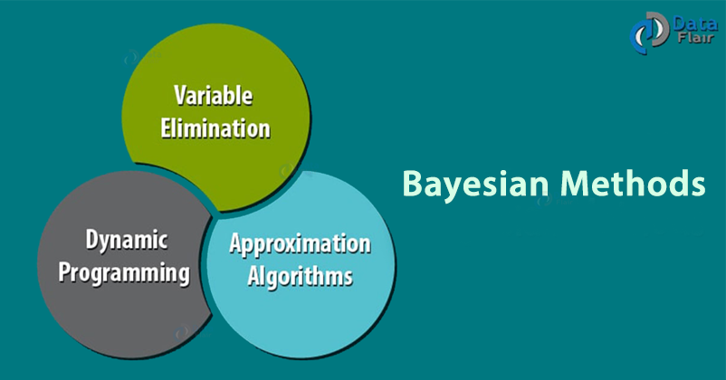
There are three different methods in a Bayesian network:
- Variable elimination
- Dynamic Programming
- Approximation algorithms
Let us discuss these Bayesian Methods one by one:
1. Variable Elimination
To do the effective marginalization, you can use Joint Probability Distribution. In this method, you can sum out irrelevant terms.
For example:
We’ll remove the variables from the inside-out. Starting with variable Xm and finishing with variable X1. Here we carry out summations right-to-left, storing intermediate results (factors) to avoid recomputation. To remove variable Xi, we start by gathering up all the factors that mention Xi and removing them from our set of factors. During the computation, the complexity of variable elimination depends on the size of the largest factor. This, in turn, depends on the order of elimination of variables. In poly tree networks, time and space complexity are linear in the size of the network.
2. Dynamic Programming
Suppose you want to calculate several margins. If you use the variable elimination algorithm, then there will be several redundant calculations. To avoid them, you can use Dynamic Programming (DP) method. It works according to the type of graphical model.
When the Bayesian Network graph is acyclic (that is, a tree), then you can use a local message-passing algorithm. This is a simple forward-backward algorithm for HMM chains. When the Bayesian Network has undirected cycles, there is a risk of double-counting by the local message-passing algorithms. To avoid this, you can convert the undirected Bayesian Network into a tree by clustering nodes together. Thus, the resulting tree is called a junction tree.
The major disadvantage of the Dynamic Programming algorithm is that it takes a longer time to run in large cluster sizes. Induced for the width of graph size refers to an increase in processing time. Minimizing the induced width of the graph is NP-hard problem. NP is a class of computational problems. You can solve this with the help of the Non-Deterministic Turing machine.
Get to know about the Top Real-world Bayesian Network Applications
3. Approximation Algorithms
Models having repetitive structures such as multivariate time-series models are used for image analysis and have a high induced width. So they take a lot of time if you try to infer them with variable elimination or Dynamic Programming algorithm.
For these models, you can also use approximation techniques. Let us see some primary approximation techniques
3.1 Variational Method
It is one of the simplest mean-field techniques used for the approximation of algorithms. It uses the rule of approximating the sum of random variables having large values using their means.
3.2 Sampling (Monte Carlo) Method
This is the simplest type of importance sampling. The general method is:
- Define samples x from P(x).
- Check samples using their likelihood P(x or y)
3.3 Loopy Belief Propagation
In this method, the actual graph applies pearl algorithm. This results in double counting. It has been observed that double-counted incidents are cancelled and offered accurate results.
3.4 Bounded Cutset Conditioning
You can break loops in the graph by instantiating subsets of the variables. This process is very slow in the case of a large cutset. To calculate this, lower bounds instantiate a subset of the cutset values.
3.5 Parametric Approximation Method
Intermediate summands in a simple and easy to understand form. For Example, Mini buckets and Boyen-Koller algorithm.
Summary
In this article, we took a brief look at different Bayesian Methods and approximation techniques for the same. We hope the information provided was useful to you.
Next, you must go through our tutorial on Bayesian Networks Inference
If you have any query related to Bayesian Methods, you can leave a comment in the section given below.
Your opinion matters
Please write your valuable feedback about DataFlair on Google


