Top Data Science Project – Sentiment Analysis Project in R
Job-ready Online Courses: Click, Learn, Succeed, Start Now!
Today, we are starting our series of R projects and the first one is Sentiment analysis. So, in this article, we will develop our very own project of sentiment analysis using R. We will make use of the tiny text package to analyze the data and provide scores to the corresponding words that are present in the dataset. In the end, you will become industry ready to solve any problem related to R programming.
Before we start, you must take a quick revision to R concepts.
R Project – Sentiment Analysis
The aim of this project is to build a sentiment analysis model which will allow us to categorize words based on their sentiments, that is whether they are positive, negative and also the magnitude of it. Before we start with our R project, let us understand sentiment analysis in detail.
What is Sentiment Analysis?
Sentiment Analysis is a process of extracting opinions that have different polarities. By polarities, we mean positive, negative or neutral. It is also known as opinion mining and polarity detection. With the help of sentiment analysis, you can find out the nature of opinion that is reflected in documents, websites, social media feed, etc. Sentiment Analysis is a type of classification where the data is classified into different classes. These classes can be binary in nature (positive or negative) or, they can have multiple classes (happy, sad, angry, etc.).
If you are not aware of the topic classification in R, here is the best guide – R Classification.
Developing our Sentiment Analysis Model in R
We will carry out sentiment analysis with R in this project. The dataset that we will use will be provided by the R package ‘janeaustenR’.
In order to build our project on sentiment analysis, we will make use of the tidytext package that comprises of sentiment lexicons that are present in the dataset of ‘sentiments’.
First, we will import the needed packages, then we will go through data cleaning and data preprocessing steps. Pre-processing of text data involves; to help remove the noise from the data, converting the text data to all lower cases, eliminating all punctuations and eradicating stop words such as “the”, “is” “and” and others. The preprocessing step is followed by tokenizing the text, which involves the decomposition of text into manageable words or terms on which sentiment can be determined.
After data preparation, sentiment lexicons will be adopted so as to score the words respectively. Lexicons are the word list that have been preprocessed and each word has been assigned sentiment polarity scores for it. These scores aid in establishing the degree of positivity or negativity of a piece of text. For instance, happy, joy will be positive while sad, anger will be negative. The addition of these scores makes it possible to measure the polarity of a rather large amount of text such as a paragraph and other documents.
Syntax:
library(tidytext)
Sentiments
Screenshot: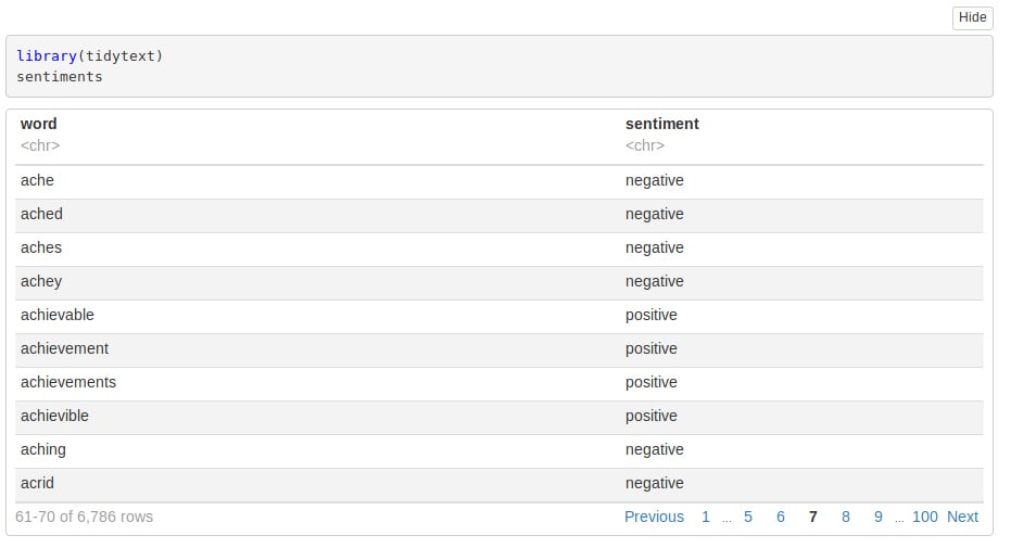
We will make use of three general purpose lexicons like –
- AFINN
- bing
- loughran
These three lexicons make use of the unigrams. Unigrams are a type of n-gram model that consists of a sequence of 1 item, that is, a word collected from a given textual data. In the AFINN lexicon model scores the words in a range from -5 to 5. The increase in negativity corresponds the negative sentiment whereas an increase in positivity corresponds the positive one. The bing lexicon model on the other hand, classifies the sentiment into a binary category of negative or positive. And finally, the loughran model that performs analysis of the shareholder’s reports. In this project, we will make use of the bing lexicons to extract the sentiments out of our data. We can retrieve these lexicons using the get_sentiments() function. We can implement this as follows –
Syntax:
get_sentiments("bing")Screenshot: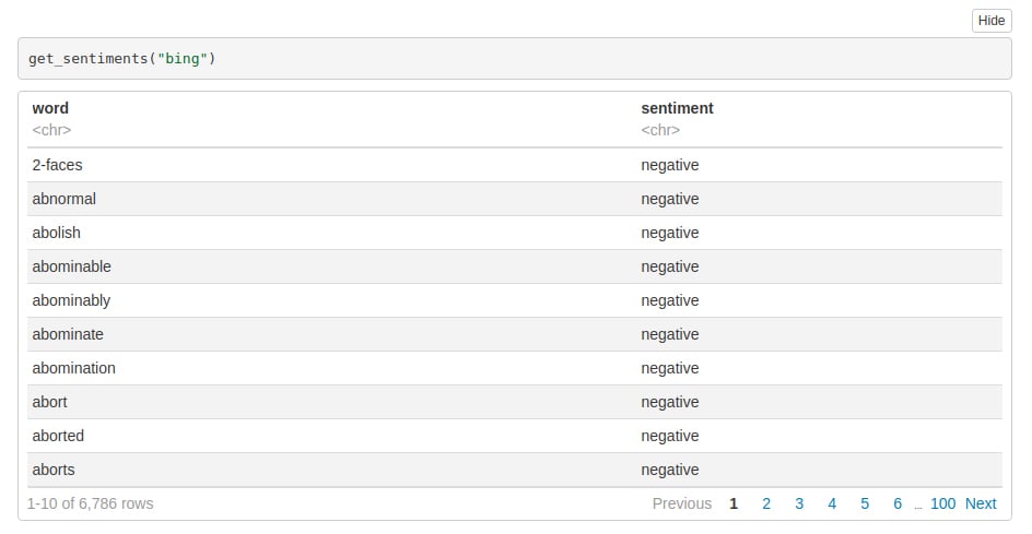
While practicing the R concepts through this project, I recommend you to start your R interview preparations also. Here are some of the best R interview questions that are mostly asked and will surely help you in the future.
Let’s continue to R sentiment analysis
Performing Sentiment Analysis with the Inner Join
In this step, we will import our libraries ‘janeaustenr’, ‘stringr’ as well as ‘tidytext’. The janeaustenr package will provide us with the textual data in the form of books authored by the novelist Jane Austen. Tidytext will allow us to perform efficient text analysis on our data. We will convert the text of our books into a tidy format using unnest_tokens() function.
Syntax:
library(janeaustenr)
library(stringr)
library(tidytext)

tidy_data <- austen_books() %>%
 group_by(book) %>%
 mutate(linenumber = row_number(),
   chapter = cumsum(str_detect(text, regex("^chapter [\\divxlc]",
                          ignore_case = TRUE)))) %>%
ungroup() %>%
unnest_tokens(word, text)
Screenshot: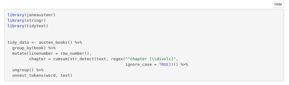
We have performed the tidy operation on our text such that each row contains a single word. Now we will make use of the “bing” lexicon to and implement filter() over the words that correspond to joy. We will use the book Sense and Sensibility and derive its words to implement out sentiment analysis model.
Syntax:
positive_senti <- get_sentiments("bing") %>%
 filter(sentiment == "positive")

tidy_data %>%
 filter(book == "Emma") %>%
 semi_join(positive_senti) %>%
 count(word, sort = TRUE)
Screenshot: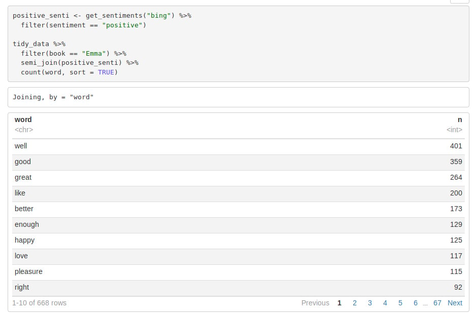
From our above result, we observe many positive words like “good”, “happy”, “love” etc. In the next step, we will use spread() function to segregate our data into separate columns of positive and negative sentiments. We will then use the mutate() function to calculate the total sentiment, that is, the difference between positive and negative sentiment.
Syntax:
library(tidyr)
bing <- get_sentiments("bing")
Emma_sentiment <- tidy_data %>%
 inner_join(bing) %>%
 count(book = "Emma" , index = linenumber %/% 80, sentiment) %>%
 spread(sentiment, n, fill = 0) %>%
 mutate(sentiment = positive - negative)
Screenshot: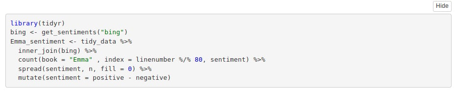
Have you checked the importance of R for Data Scientists?
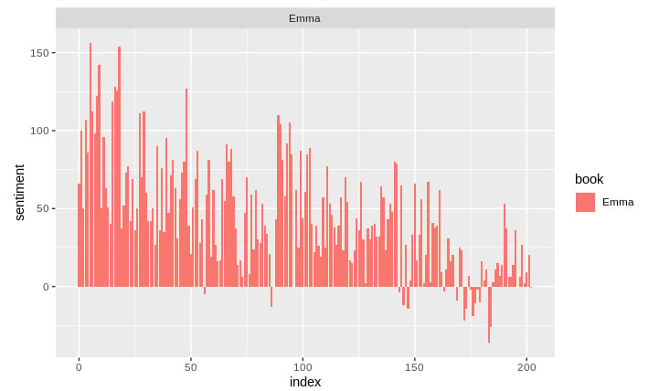
In the next step, we will visualize the words present in the book “Emma” based on their corrosponding positive and negative scores.
Syntax:
library(ggplot2)

ggplot(Emma_sentiment, aes(index, sentiment, fill = book)) +
 geom_bar(stat = "identity", show.legend = TRUE) +
 facet_wrap(~book, ncol = 2, scales = "free_x")
Screenshot: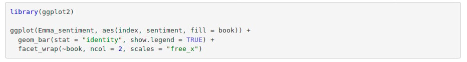
Let us now proceed towards counting the most common positive and negative words that are present in the novel.
counting_words <- tidy_data %>%
 inner_join(bing) %>%
 count(word, sentiment, sort = TRUE)
head(counting_words)
Screenshot: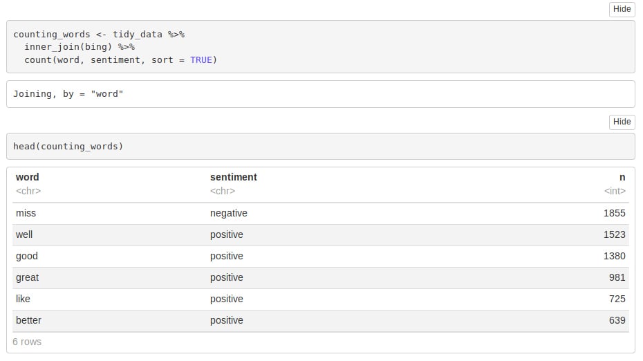
In the next step, we will perform visualization of our sentiment score. We will plot the scores along the axis that is labeled with both positive as well as negative words. We will use ggplot() function to visualize our data based on their scores.
Don’t forget to check our latest guide on data visualization using R.
Syntax:
counting_words %>%
 filter(n > 150) %>%
 mutate(n = ifelse(sentiment == "negative", -n, n)) %>%
 mutate(word = reorder(word, n)) %>%
 ggplot(aes(word, n, fill = sentiment))+
 geom_col() +
 coord_flip() +
 labs(y = "Sentiment Score")
Screenshot: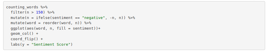
In the final visualization, let us create a wordcloud that will delineate the most recurring positive and negative words. In particular, we will use the comparision.cloud() function to plot both negative and positive words in a single wordcloud as follows:
Syntax:
library(reshape2)
library(wordcloud)
tidy_data %>%
 inner_join(bing) %>%
 count(word, sentiment, sort = TRUE) %>%
 acast(word ~ sentiment, value.var = "n", fill = 0) %>%
 comparison.cloud(colors = c("red", "dark green"),
          max.words = 100)
Screenshot: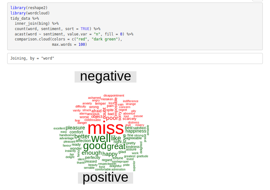
This word cloud will enable us to efficiently visualize the negative as well as positive groups of data. Therefore, we are now able to see the different groups of data based on their corresponding sentiments. You can experiment with several other datasets like tweets in order to gain a comprehensive insight into sentiment analysis. At any point, if you feel you need to revise your R learning, reach out to DataFlair. We have a series of 120+ FREE R Tutorials that will help you like anything.
Summary
In this blog, we went through our project of sentiment analysis in R. Then we learnt about the concept of sentiment analysis and implemented it over the dataset of Jane Austen’s books. We were able to delineate it through various visualizations after we performed data wrangling on our data. We used a lexical analyzer – ‘bing’ in this instance of our project. Furthermore, we also represented the sentiment score through a plot and also made a visual report of wordcloud.
Hope you enjoyed this R Sentiment Analysis Project. Drop your queries through comments, we will definitely help.
Did you like our efforts? If Yes, please give DataFlair 5 Stars on Google


How to perform sentiment analysis on sentences? Any easy example..
good
I’m data science masters student @ university of Gondar, Ethiopia. can you help me by giving all the coddes and the documentation parts of this “sentiment analysis model” to use as a reference for my papers
can you help me by giving all the coddes and the documentation parts of this “sentiment analysis model” for my mini projrct
Hello Belayneh,
The codes are available in the article with their detailed description. Kindly, go through the full article thoroughly. I am sure you will find the codes and documents which you are looking for.
What if we have a positive or negative word phrased after the opposite one?
I’m data science masters student can you help me by giving all the codes and the documentation parts of this “sentiment analysis model” to use as a reference for my papers
can you help me by giving all the coddes and the documentation parts of this “sentiment analysis model” for my project
Can You Help me in Automatic License Number Plate Recognition System please
count(book = “Emma” , index = linenumber %/% 80, sentiment)
why index is taken as linenumber %/% 80?
Any specific reason behind that/
it is a modular division, here integer divide x by y and return the remainder.
Hi DataFlair Team,
You have used %>% on many places. What does it actually do?
It’s called the “pipe” operator. It is not in base R, but is included in packages such as the tidyverse. The pipe allows you to take the result of one piece of code and feed it to the next piece as the first argument.
Instead of:
my_name % print()
You do this because it is sometimes easier than saving things as an object (e.g. my_name).
Consider:
huge_data_frame %>%
select(thingy == “big”) %>%
filter(smell == “nasty”)
Here you are piping data quickly through functions, with the output of one being the input of another.
Are you guys using RStudio for coding ?
Bonjour.J’aimerais bien avoir si possible le lien github du projet si il est public.Merci
Good learning. Thank you for sharing the knowledge.
Je ne pense pas ! Le site a toutes les explications de base. Vous pouvez essayer s’il existe un code source disponible dans Github, bienvenue !
can someone help me with this error
ungroup() %>%
unnest_tokens(word, Text)
Error in ungroup(.) : could not find function “ungroup”
help me with this error plz
ungroup() %>%
unnest_tokens(word, Text)
Error in ungroup(.) : could not find function “ungroup”
Hi sam marsy!
To stop getting the error message, try loading the dplyr package just after the tidytext package.
library(dplyr)