How to Create Generalized Linear Models in R – The Expert’s Way!

Earlier we have discussed Graphical Models. Today, DataFlair has come up with a new and very important topic that is R Generalized Linear Models. We will see what exactly R Generalized linear models are and how can you create them. Also, we will discuss Logistic and Poisson Regression in detail. So, let’s start the tutorial –

What are the Generalized Linear Models in R?

Generalized Linear Models in R are an extension of linear regression models allow dependent variables to be far from normal. A general linear model makes three assumptions –

• Residuals are independent of each other.
• Residuals are distributed normally.
• Model parameters and y share a linear relationship.

A Generalzed Linear Model extends on the last two assumptions. It generalizes the possible distributions that the residuals share to a family of distributions known as the exponential family.

For Example – Normal, Poisson, Binomial

In R, we can use the function glm() to work with generalized linear models in R. Thus, the usage of glm() is like that of the function lm() which we before used for much linear regression. We use an extra argument family. That is to describe the error distribution. And link function to be used in the model to show the main difference.

GLM are fit using the glm( ) function. The form of the glm function is –

glm(formula, family=familytype(link=linkfunction), data=)

a. Logistic Regression

We implement the Logistic Regression method for fitting the regression curve y = f(x). Here, y is a categorical variable.  

It is a classification algorithm. This model gives out an outcome which is binary in nature. We also use dummy variables to indicate the absence or presence of an effect on the overall result of the model. 

The response variable, also known as the dependent variable is categorical in nature. It measures the outcome of the binary response variable. Thus, it actually measures the probability of a binary response.

We use the following R glm() function for modeling our logistic regression method.

> glm( response ~ explanantory_variables , family=binomial)

b. Poisson Regression

Data is often collected in counts. Hence, many discrete response variables have counted as possible outcomes. While binomial counts are the number of successes in a fixed number of trials, n.

Poisson counts are the number of occurrences of some event in a certain interval of time (or space). Apart from this, Poisson counts have no upper bound and binomial counts only take values between 0 and n. 

To perform logistic regression in R, we use the command:

> glm( response ~ explanantory_variables , family=poisson)

Don’t forget to check our leading blog on Graphical Models Applications

How to Create a Generalized Linear Model in R

In order to create our first linear model, we will make apply linear regression over the ‘car’ dataset.

Code:

#Author DataFlair
data(cars)
head(cars)
scatter.smooth(x=cars$speed, 
         y=cars$dist, 
         main="Dist ~ Speed")

Output:

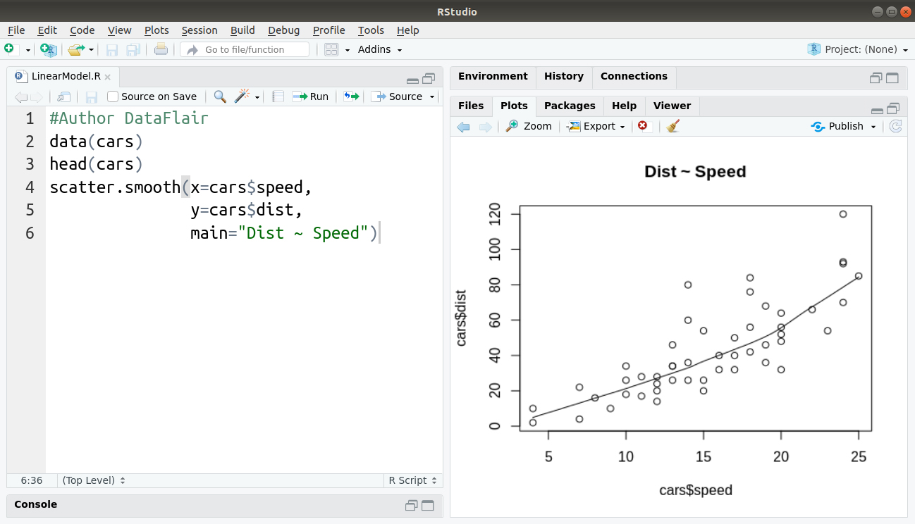
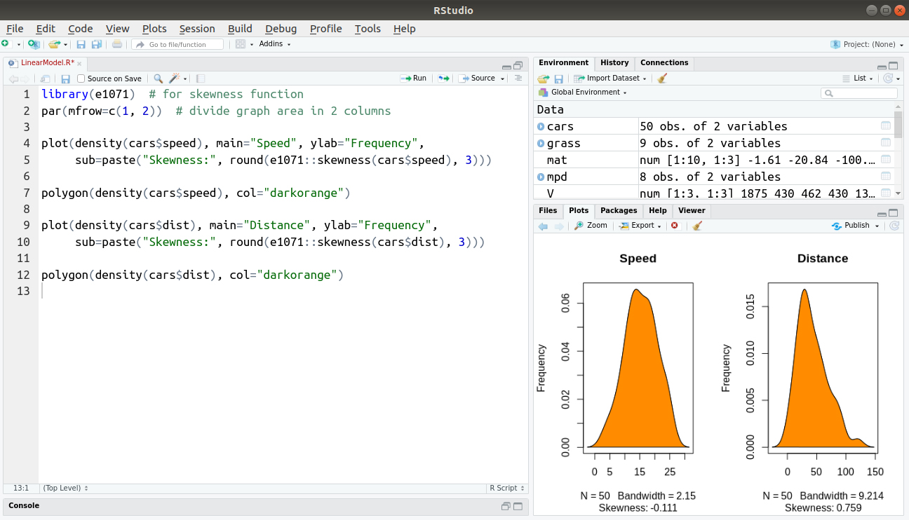
One of the most important steps before implementing linear regression is to check if the dependent variable (distance) is close to normal. We will assess this by visualizing a density plot as follows –

Code:

library(e1071) # for skewness function
par(mfrow=c(1, 2)) # divide graph area in 2 columns

plot(density(cars$speed), main="Speed", ylab="Frequency", 
   sub=paste("Skewness:", round(e1071::skewness(cars$speed), 3)))

polygon(density(cars$speed), col="darkorange")

plot(density(cars$dist), main="Distance", ylab="Frequency", 
   sub=paste("Skewness:", round(e1071::skewness(cars$dist), 3)))

polygon(density(cars$dist), col="darkorange")

Output:

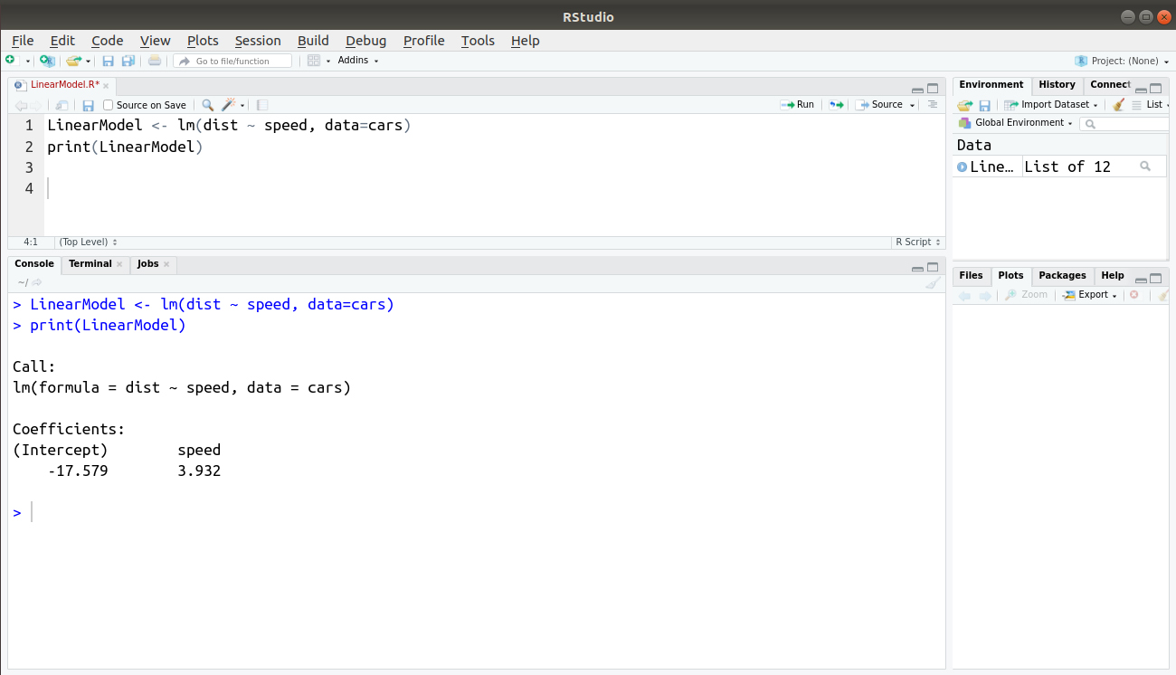
Code:

LinearModel <- lm(dist ~ speed, data=cars) 
print(LinearModel)

Output:

This is the right time to learn the most important topic of R programming – R Data Visualization. Check this and comment us your learning experience

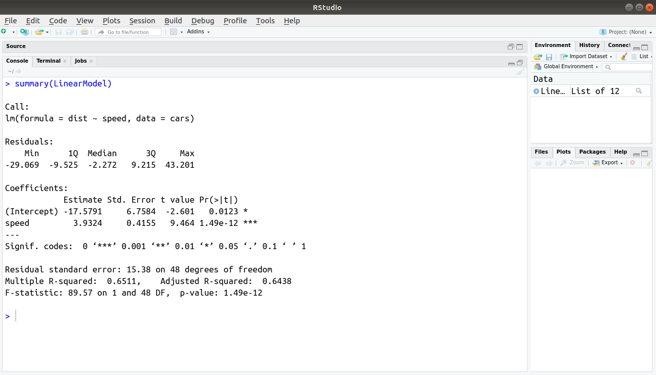
Now, with the help of summary() function, we will understand the summary statistics associated with our model –

Code:

summary(LinearModel)

Output:

Another type of linear modeling is survival analysis. You can learn about it in our tutorial on Survival Analysis in R. 

Summary

We learned the concept of generalized linear model in R. Hope after completing this, you are able to create a generalized linear model. If still in doubt, comment below. DataFlair will surely help you.

Happy Learning😊