R Decision Trees – The Best Tutorial on Tree Based Modeling in R!
Job-ready Online Courses: Click, Learn, Succeed, Start Now!
In this tutorial, we will cover all the important aspects of the Decision Trees in R. We will build these trees as well as comprehend their underlying concepts. We will also go through their applications, types as well as various advantages and disadvantages.
Let’s now begin with the tutorial on R Decision Trees.
What is R Decision Trees?
Decision Trees are a popular Data Mining technique that makes use of a tree-like structure to deliver consequences based on input decisions. One important property of decision trees is that it is used for both regression and classification. This type of classification method is capable of handling heterogeneous as well as missing data. Decision Trees are further capable of producing understandable rules. Furthermore, classifications can be performed without many computations.
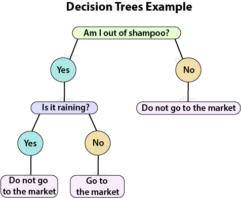
As mentioned above, both the classification and regression tasks can be performed with the help of Decision Trees. You can perform either classification or regression tasks here. Decision Trees can be visualised as follows:
Applications of Decision Trees
Decision Trees are used in the following areas of applications:
- Marketing and Sales – Decision Trees play an important role in a decision-oriented sector like marketing. In order to understand the consequences of marketing activities, organisations make use of Decision Trees to initiate careful measures. This helps in making efficient decisions that help the company to reap profits and minimize losses.
- Reducing Churn Rate – Banks make use of machine learning algorithms like Decision Trees to retain their customers. It is always cheaper to keep customers than to gain new ones. Banks are able to analyze which customers are more vulnerable to leaving their business. Based on the output, they are able to make decisions by providing better services, discounts as well as several other features. This ultimately helps them to reduce the churn rate.
- Anomaly & Fraud Detection – Industries like finance and banking suffer from various cases of fraud. In order to filter out anomalous or fraud loan applications, information and insurance fraud, these companies deploy decision trees to provide them with the necessary information to identify fraudulent customers.
- Medical Diagnosis – Classification trees identifies patients who are at risk of suffering from serious diseases such as cancer and diabetes.
How to Create Decision Trees in R
The Decision Tree techniques can detect criteria for the division of individual items of a group into predetermined classes that are denoted by n.
In the first step, the variable of the root node is taken. This variable should be selected based on its ability to separate the classes efficiently. This operation starts with the division of variable into the given classes. This results in the creation of subpopulations. This operation repeats until no separation can be obtained.
A tree exhibiting not more than two child nodes is a binary tree. The origin node is referred to as a node and the terminal nodes are the trees.
To create a decision tree, you need to follow certain steps:
1. Choosing a Variable
The choice depends on the type of Decision Tree. Same goes for the choice of the separation condition.
In the case of a binary variable, there is only one separation whereas, for a continuous variable, there are n-1 possibilities.
The separation condition is as follows:
X <= mean(xk, xk+1)
After finding the best separation, the operation is repeated to increase discrimination among the nodes.
The density of the node is its ratio of the individuals to the entire population.
After finding the best separation, classes are split into child nodes. We derive a variable out of this step. We choose the best separation criteria as:
The X2 Test – For testing the independence of variables X and Y, we use X2, only if:
Oij provides us with the left-hand side of the equality symbol and Tij provides the term on the right, independence test of X and Y is X2.
This degree of freedom is calculated as:
p = (no. of rows – 1) * (no. of columns – 1)
The Gini Index – With this test, we measure the purity of nodes. All types of dependent variables use it and we calculate it as follows:
In the preceding formula: fi, i=1, . ., p, corresponds to the frequencies in the node of the class p that we need to predict.
With an increase in distribution, the Gini index will also increase. However, with the increase in the purity of the node, the Gini index decreases.
Wait a minute! Have you checked – Logistic Regression in R
2. Assigning Data to Nodes
After the construction is completed and the decision criteria is established, every individual is assigned one leaf. The independent variable determines this assignment. This leaf is assigned only if the cost of the assignment is higher than another leaf to the present class.
3. Pruning the Tree
In order to remove irrelevant nodes from the trees, we perform pruning. If a large-sized tree is created, followed by automatic pruning, then we refer to that algorithm as good. We perform cross-validation and aggregate the error rates for all the subtrees in order to select the best one. Furthermore, we shorten the deep tree branches to limit the creation of the small nodes.
Common R Decision Trees Algorithms
There are three most common Decision Tree Algorithms:
- Classification and Regression Tree (CART) investigates all kinds of variables.
- Zero (developed by J.R. Quinlan) works by aiming to maximize information gain achieved by assigning each individual to a branch of the tree.
- Chi-Square Automation Interaction Detection (CHAID) – It is reserved for the investigation of discrete and qualitative independent and dependent variables.
1. Classification and Regression Tree (CART)
CART is the most popular and widely used Decision Tree. The primary tool in CART used for finding the separation of each node is the Gini Index.
Performance and Generality are the two advantages of a CART tree:
- Generality – In Generality, the categories can be either definite or indefinite. Furthermore, this type of CART can be used for classification as well as regression problems. This can, however, be done with appropriate splitting criteria.
Generality is increased through an increase in the capacity to process missing values through replacement of a variable with an equally splitting variable. - Performance – The performance of CART is dependent on the pruning mechanism. By proceeding with the continuation of the node splitting process, we are able to construct the largest tree (that is possible). Continuing node splitting process constructs largest trees (as large as possible). The algorithm then deduces many nested subtrees by successive pruning operations.
CART has the following drawbacks as well:
- CART produces a narrow and deep complex decision trees owing to its binary structures. As a result, the readability of the trees is poor in some cases.
- CART trees hold the favour of variables that possess the largest categories. Therefore, they are biased in nature which further reduces reliability.
You must definitely have a look at Binomial and Poisson Distribution in R
2. Chi-Square Automation Interaction Detection (CHAID)
CHAID was developed as an early Decision Tree based on the 1963 model of AID tree. As opposed to CHAID, it does not substitute the missing values with the equally reducing values. All the missing values are taken as a single class which facilitates merging with another class. For finding the significant variable, we make use of the X2 test. This is only valid for qualitative or discrete variables. We create CHAID in the following steps:
- The cross-tabulation of categories is carried out by X2 which groups them in k-categories. Furthermore, the response variable for X holds 3 categories. The categories of X cross-tabulates them with the k categories of the response variable for every X having at least 3 categories.
- You need to repeat the above step until all the pairs of categories have a significant X2, or until no more than two categories exist. If there is an existence of frequency below the minimum value, the collaboration is carried out with a category that is closest to X2.
- The groupings are performed to the variables into their corresponding classes. If there are any missing values present then it is assumed as a category. After the completion, CHAD merges it with another category.
- We now obtain the probability of X2 of the best table. We multiply this with Bonferroni correction, obtain the number of possibilities to cluster m categories into g groups with this coefficient. Furthermore, its product by the probability that is associated with X2 prevents evaluation of the significance of multiple values.
- With CHAID, we select the most significant variable for X2. This variable possesses the lowest probability. If it is below the given limit, then we perform division of the node into child nodes that are equal to the categories of variables required for grouping.
CHAID trees are wider than deeper. Furthermore, there is no pruning function available for it. Also, the construction halts when the largest tree is created.
With the help of CHAID, we can transform quantitative data into a qualitative one.
Take a deep dive into Contingency Tables in R
Guidelines for Building Decision Trees in R
Decision Trees belong to the class of recursive partitioning algorithms that can be implemented easily. The algorithm for building decision tree algorithms are as follows:
- Firstly, the optimized approach towards data splitting should be quantified for each input variable.
- The best split is to be selected, followed by the division of data into subgroups that are structured by the split.
- After a subgroup is picked, we repeat step 1 for each of the underlying subgroups.
- The splitting is to be continued until you achieve the split that belongs to the same target variable value until you encounter a halt.
This halt condition may pose complications in the form of a statistical significance test or the least record count. Since Decision Trees are non-linear predictors, the decision boundaries between the target class are also non-linear. Based on the number of splits, the non-linearities change.
Some of the important guidelines for creating decision trees are as follows:
- The variables are only present in a single split. Therefore, if the variable splits an individual by itself, Decision Trees may have a faulty start. Therefore, trees require good attributes to boost their start.
- The weak learners can produce considerable changes to the tree in the form of its structure and behaviour. In order to understand the value of winning split, we examine the competitors.
- The bias of the Decision Trees is directed towards the selection of categorical variables that comprise the greater leaver. If there are greater levels, then we can use the cardinal penalty to reduce the number of levels.
- Data can often get exhausted in trees before a good fit is achieved. Since every split of the tree reduces the records, the further splits only possess fewer records.
- The accuracy of the individual trees is not as high as compared to other algorithms. Variable Selection forwarding and constant node splitting are the main reasons behind this.
You must learn about the Non-Linear Regression in R
Decision Tree Options
- Maximum Depth – This defines the number of levels of depth that a tree can be shaped.
- Minimum Number of Records in Terminal Nodes – This is useful for determining the least number of records that a terminal node allows. If the split causes the results to be below the threshold level, then the split is not carried out.
- Outputting Differentiated Clusters
- Minimum Number of Records in Parent Node – This is similar to minimum records in terminal nodes that we discussed above. However, the difference lies in the application where a split actually occurs. If the records are much lesser than the number of records that are specified, then the split process is halted.
- Bonferroni Correction – The adjustments are carried for various comparisons where the chi-square statistic for a categorical input is compared with the target test.
Get a deep insight into the Chi-Square Test in R with Examples
How to Build Decision Trees in R
We will use the rpart package for building our Decision Tree in R and use it for classification by generating a decision and regression trees. We will use recursive partitioning as well as conditional partitioning to build our Decision Tree. R builds Decision Trees as a two-stage process as follows:
- Performing the identification of a unique variable that splits the variable into groups.
- It applies the above process for each subgroup until the subgroup reach to the minimum size or no improvement in a subgroup is shown.
We will make use of the popular titanic survival dataset. We will first import our essential libraries like rpart, dplyr, party, rpart.plot etc.
#Author DataFlair
library(rpart)
library(readr)
library(caTools)
library(dplyr)
library(party)
library(partykit)
library(rpart.plot)
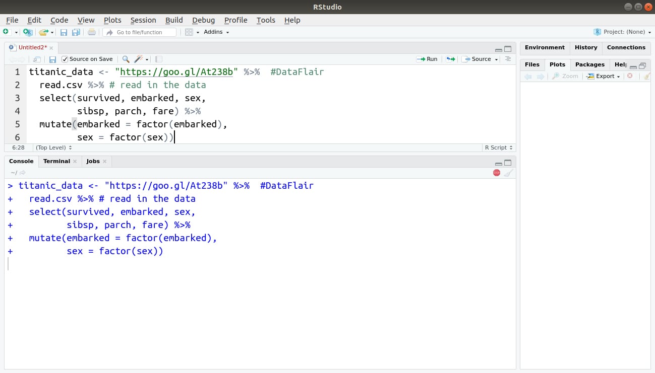
After this, we will read our data and store it inside the titanic_data variable.
titanic_data <- "https://goo.gl/At238b" %>%  #DataFlair
  read.csv %>% # read in the data
  select(survived, embarked, sex,
         sibsp, parch, fare) %>%
  mutate(embarked = factor(embarked),
         sex = factor(sex))
Output:
After this, we will split our data into training and testing sets as follows:
set.seed(123)
sample_data = sample.split(titanic_data, SplitRatio = 0.75)
train_data <- subset(titanic_data, sample_data == TRUE)
test_data <- subset(titanic_data, sample_data == FALSE)
Output:

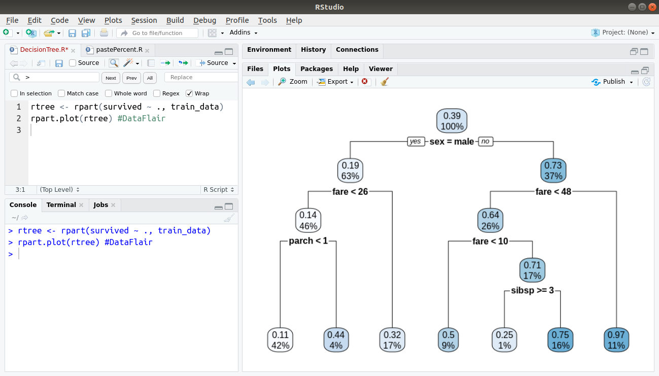
Then, we will proceed to plot our Decision Tree using the rpart function as follows:
rtree <- rpart(survived ~ ., sample_data$train_data)
rpart.plot(rtree)
Output:
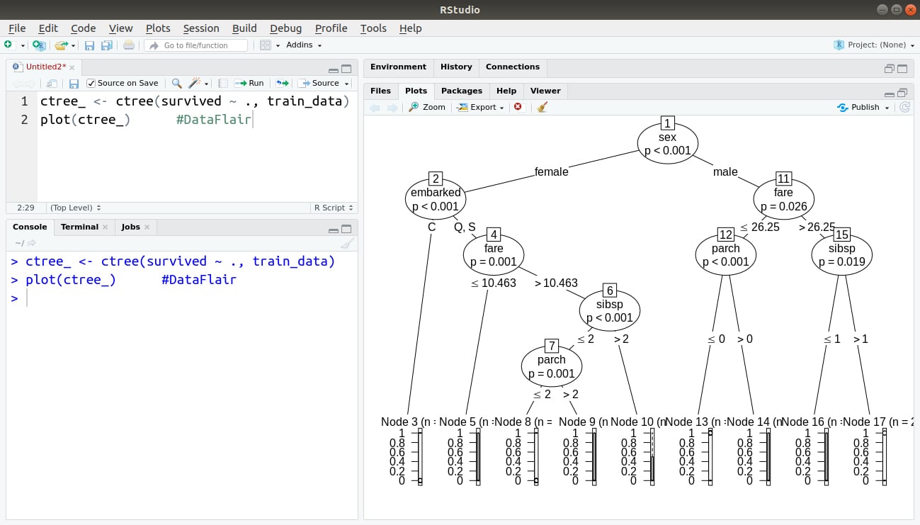
We will also plot our conditional parting plot as follows:
ctree_ <- ctree(survived ~ ., train_data)
plot(ctree_)
Output:
Let’s master the Survival Analysis in R Programming
Prediction by Decision Tree
Similar to classification, Decision Trees can also be used for prediction. In order to carry out the latter, it changes the node split criterion. The aim of implementing this is:
- The dependent variable should possess a smaller variance in their child nodes. This is in contrast with the parent node.
- The mean of the dependent variable must be different from their child node.
You should be able to select the child nodes that are able to reduce intra-class variance and amplify inter-class variance. For example, a CHAID tree. Given an input of 163 countries, it groups them into five clusters based on the differences that their citizens share on the basis of their GNP. After the groups are made, there is another split based on life expectancy.
Advantages of R Decision Trees
Decision Trees are highly popular in Data Mining and Machine Learning techniques. Following are the advantages of Decision Trees:
- Decision Trees allow you to comprehend results which convey explicit conditions based on the original variables. Since Decision Trees do not require a lot of computation for processing, the IT staff can easily program the model without any hassle. The calculations comprise numerical comparisons that delineate whether the model is qualitative or quantitative in nature.
- Decision Trees are non-parametric in nature. Therefore, they do not follow any pattern of the probability distribution. Furthermore, the nature of these variables can be collinear.
- Extreme individuals do not affect Decision Trees. Such instances can be isolated in groups of minor nodes as they do not affect classification on a larger scale.
- As opposed to other ML algorithms that suffer from missing data, Decision Trees can very well handle it. With the help of CHAID, Decision Trees can handle missing variables by treating them as an isolated category or merging them into another.
- Trees like CART and C5.0 allow the variables to be handled directly. These type of variables are continuous, discrete and qualitative in nature.
- There are various visual representations provided by the Decision Tree for making decisions. This enhances communication and the branches contribute towards greater decision making.
Get to know about the Machine Learning Techniques with Python
Disadvantages of R Decision Trees
Decision Trees possess the following disadvantages:
- According to the definition, the nodes at the level n+1 are dependent on the definition of n level. Therefore, if the condition at level n is true, only then n+1 will be true. Otherwise, it will be false.
- The tree is constrained to local optima. It cannot detect global optima. The values are evaluated sequentially and not simultaneously. Due to this, the node will never revise its choice of division subsequently. The tree detects local, not global optima. It evaluates all the independent variables sequentially, not simultaneously.
- If the variable is located near the top of the true, its modification can alter the structure of the entire tree. This can be overcome with oversampling but it will reduce the readability of the model.
This was all about our tutorial on Decision Trees. We hope you liked it and gained useful information.
Summary
In the above tutorial, we understood the concept of R Decision Trees. We further discussed the various applications of these trees. Furthermore, we learnt how to build these trees in R. We also learnt some useful algorithms such as CART and CHAID. We went through the advantages and disadvantages of R trees.
Don’t forget to check out the article on Random Forest in R Programming
If you have any query, we will be glad to solve them for you.
Did you like this article? If Yes, please give DataFlair 5 Stars on Google


Respected
Please share R coding for decision tree so I can understood the concept with coding also
Thanks for the great introduction to the various kinds of trees, the article would be even better if it included how to find each tree (CART, C5.0, and CHAID) in R, i.e. which library includes which tree and how to select it.
Can we get weights of the variables used for dividing the nodes from a decision tree using Rpart?
How to check which predictors are significant for splitting the whole data in decision tree?