R Linear Regression Tutorial – Door to master its working!
Expert-led Courses: Transform Your Career – Enroll Now
In this tutorial, we are going to study about the R Linear Regression in detail. First of all, we will explore the types of linear regression in R and then learn about the least square estimation, working with linear regression and various other essential concepts related to it.
What is Linear Regression?
Regression analysis is a statistical technique for determining the relationship between two or more than two variables. There are two types of variables in regression analysis – independent variable and dependent variable. Independent variables are also known as predictor variables. These are the variables that do not change. On the other side, the variables whose values change are known as dependent variables. These variables depend on the independent variables. Dependent variables are also known as response variables.
With the help of linear regression, we carry out a statistical procedure to predict the response variable based on the input of the independent or predictor variables.
Linear Regression is of the following two types:
- Simple Linear Regression – Based on the value of the single explanatory variable, the value of the response variable changes.
- Multiple Linear Regression – The value is dependent upon more than one explanatory variables in case of multiple linear regression.
Some common examples of linear regression are calculating GDP, CAPM, oil and gas prices, medical diagnosis, capital asset pricing, etc.
Wait! Have you checked – OLS Regression in R
1. Simple Linear Regression in R
Simple linear regression is used for finding the relationship between the dependent variable Y and the independent or predictor variable X. Both of these variables are continuous in nature. While performing simple linear regression, we assume that the values of predictor variable X are controlled. Furthermore, they are not subject to the measurement error from which the corresponding value of Y is observed.
The equation of a simple linear regression model to calculate the value of the dependent variable, Y based on the predictor X is as follows:
yi = β0 + β1x + ε
Where the value of yi is calculated with the input variable xi for every ith data point;
The coefficients of regressions are denoted by β0 and β1;
The ith value of x has εi as its error in the measurement.
Regression analysis is implemented to do the following:
- With it, we can establish a linear relationship between the independent and the dependent variables.
- The input variables x1, x2….xn is responsible for predicting the value of y.
- In order to explain the dependent variable precisely, we need to identify the independent variables carefully. This will allow us to establish a more accurate causal relationship between these two variables.
Do you know about Principal Components and Factor Analysis in R
2. Multiple Linear Regression in R
In many cases, there may be possibilities of dealing with more than one predictor variable for finding out the value of the response variable. Therefore, the simple linear models cannot be utilised as there is a need for undertaking multiple linear regression for analysing the predictor variables.
Using the two explanatory variables, we can delineate the equation of multiple linear regression as follows:
yi = β0 + β1x1i + β2x1i + εi
The two explanatory variables x1i and x1i, determine yi, for the ith data point. Furthermore, the predictor variables are also determined by the three parameters β0, β1, and β2 of the model, and by the residual ε1 of the point i from the fitted surface.
General Multiple regression models can be represented as:
yi = Σβ1x1i + εi
Least Square Estimation
While the simple and multiple regression models are capable of explaining the linear relationship between variables, they are incapable of explaining a non-linear relationship between them.
The method of least squares is used for defining both the multiple as well as simple linear equations. We further calculate the unknown parameters with the help of least square estimation method.
In order to minimise the sum of squares for determining the best fit, we make use of the Least Square Estimation method. The errors in the least square estimation are generated due to certain deviations in the observed points which are far from the proposed one. This deviation is residual in nature.
We can calculate the sum of squares of the residuals with the following equation:
SSR=Σe2=Σ(y-(b0+b1x))2
Where e is the error, y and x are the variables, and b0 and b1 are the unknown parameters or coefficients.
You must definitely check the Chi-Square Test in R
Checking Model Adequacy
For making the predictions, we make use of the Regression Models. For making the right predictions, the adequacy of these models is first assessed.
We use the R Squared and Adjusted R Squared methods for assessing the model adequacy.
The greater values of R-Square represent a robust correlation between the independent and the dependent variables. A low value, on the contrary, represents a weak regression model by which we infer that the model is not apt at making required predictions. The value of R ranges from 0 to 1. The end-point 0 points out no correlation between sample variables. Whereas, 1 means an exact linear relationship between the two variables.
R Squared can be calculated as follows:
R2 = 1 – (SSR/SST)
Where SST stands for Sum of Squares of Total and SSR stands for Sum of Squares of Regression. These two combine to form the total sums of the squares of errors.
For adding an explanatory variable to the regression model, the adjusted R-Squared is used. The number of explanatory variables affects the value of the adjusted R-Squared. However, there is an addition of statistical penalty for each new predictor variable that is present in the regression model.
Just like the R-Squared, the adjusted R Squared can be used for the calculation of the proportion of variation that is cased by the explanatory variables.
Adjusted R Squared can be calculated as:
R2 = R2 – [k(1-R2)/(n-k-1)]
Here, n represents the number of observations and k represents the number of parameters.
Let’s quickly revise the Matrix Function in R
Regression Assumptions
When building a regression model, statisticians make some basic assumptions to ensure the validity of the regression model.
These are:
- Linearity – With this, there is an assumption of a linear relationship between the dependent and the independent variables. Since the predictor variables are treated like fixed values, the linearity is based on restriction of the parameters. Assume a linear relationship between the dependent and independent variables because it treats the predictor variables as fixed values (see above), linearity is really only a restriction on the parameters.
- Independence – This assumes that the errors of the response variables are uncorrelated with each other.
- Homoscedasticity – In homoscedasticity, the response variables possess common variances in their errors. This is completely independent of the value of predictor variables. However, in practice, this does not hold valid as the errors can be heteroscedastic. This happens when the response variable varies over a wider scale.
- Normality – In normality, the collected samples hold a normal distribution of errors.
The regression model may be insufficient for making predictions if we violate any of these assumptions.
Note: Complexity of a regression model increases with an increasing number of parameters.
Multicollinearity
In multicollinearity, we refer to redundancy. There exists a non-linear relationship between the variables which ultimately leads to inaccuracies in the parameter estimation. This takes place when two or more variables exhibit an exact or approximate relationship that is with respect to the dependent variable.
Multicollinearity can be detected by calculating VIF as follows:
VIF = 1/ (1-Ri2)
In the above equation, the regression coefficient is represented by Ri for the independent variable.
In the regression model, multicollinearity is identified when significant change is observed in estimated regression coefficients while adding or deleting explanatory variables or when VIF is high (5 or above) for the regression model.
Following are some impacts of multicollinearity:
- The regression coefficients are estimated wrongly.
- There is a constraint on our ability to estimate the standard errors as well as the coefficients.
- It is difficult to assess the estimation of an accurate manner owing to the large variances as well as covariances in the OLS for the variables that share a proximate relation.
- There is a higher probability of accepting the null hypothesis due to larger standard errors that are present.
- T-test deflation and degradation takes place because of model predictability.
We have seen the effects of multicollinearity. So if possible, remove it using the following manner:
- Specifying the regression model again.
- The estimation of the coefficients is undertaken with the help of prior information or restrictions.
- Incrementing the sample size or accumulating new data.
Don’t forget to explore the Hypothesis Testing in R
Working with R Linear Regression
In order to observe and establish a correlation between the two variables; X, and Y, we use scatterplots and other evaluation criteria like the Pearson Coefficient. When this relationship is established, we are able to predict Y based on the input value provided by X.
Y is the independent or explanatory variable. Therefore, with a change in X, Y is also expected to change in the form of a response. In order to check if the data is scattered linearly, we plot scatterplots that help us to validate the linear pattern.
The following equation is of linear regression:
Y = mx + b
In the above equation, m is the slope, that represents the change in y over the change in x. b here is the intercept on the y-axis. Furthermore, with the estimation of Y, we can calculate the slope through the correlation between X and Y.
Furthermore, the slope can be calculated with the multiplication of the correlation between the X and Y variable and their division with the standard deviation of Y values by the standard deviation of x-values. Where, m is the slope of the line(change in y over the change in x) and b is the y-intercept(that place on the y-axis where the value of x is 0). When the value of Y is estimated, the slope is then calculated through the multiplication between X and Y as well as by carrying out the division of standard deviation of y-values by the standard deviation of x-values.
Building a Linear Regression Model
The process of performing linear regression involves complex calculations owing to the number of variables. With the help of R, you can implement inbuilt functions that allow you to perform linear regression easily.
Using common software tools, statisticians can implement various statistical tools. We will now learn how to implement a linear regression model using R.
In order to build our linear regression model, we will make use of the ‘cars’ dataset and analyze the relationship between the variables – speed and distance.
1. Importing the Dataset
Import the dataset in R as follows:
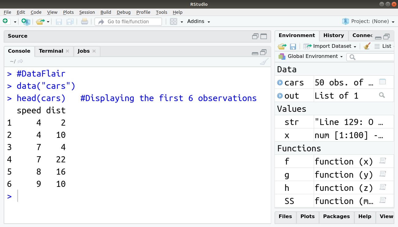
> #DataFlair
> data("cars")
> head(cars)   #Displaying the first 6 observations
Output:
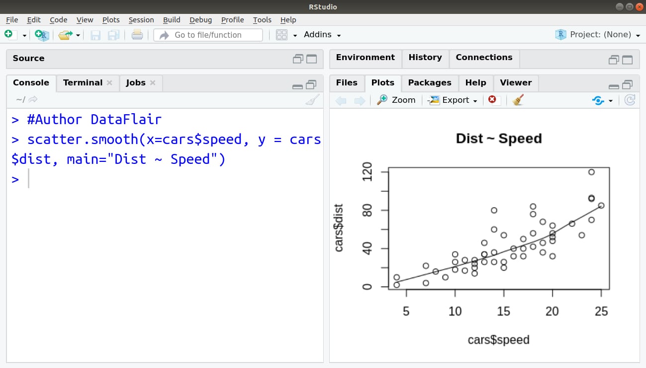
2. Visualising Linearity using Scatterplots
In order to visualise the linear relationship between independent and dependent variables, that is, distance and speed respectively, we delineate a Scatterplot. This can be done using the scatter.smooth() function:
> #Author DataFlair
> scatter.smooth(x=cars$speed, y = cars$dist, main="Dist ~ Speed")
Output:
3. Measuring Correlation Coefficient
Correlation is a statistical measure of finding out linear dependence between the two variables. The values of the correlation coefficient range between -1 to +1. There can be two types of correlation – Positive Correlation and Negative Correlation.
In positive correlation, the value of one variable will increase with an increment in the other value or decrease with reduction in the other. This value will be closer to +1.
In the case of negative correlation, the value of the variable will decrease with an increase in another variable and increase with a decrease in other. Therefore, there is an inverse relationship between the two variables. The value of this correlation coefficient will be closer to -1.
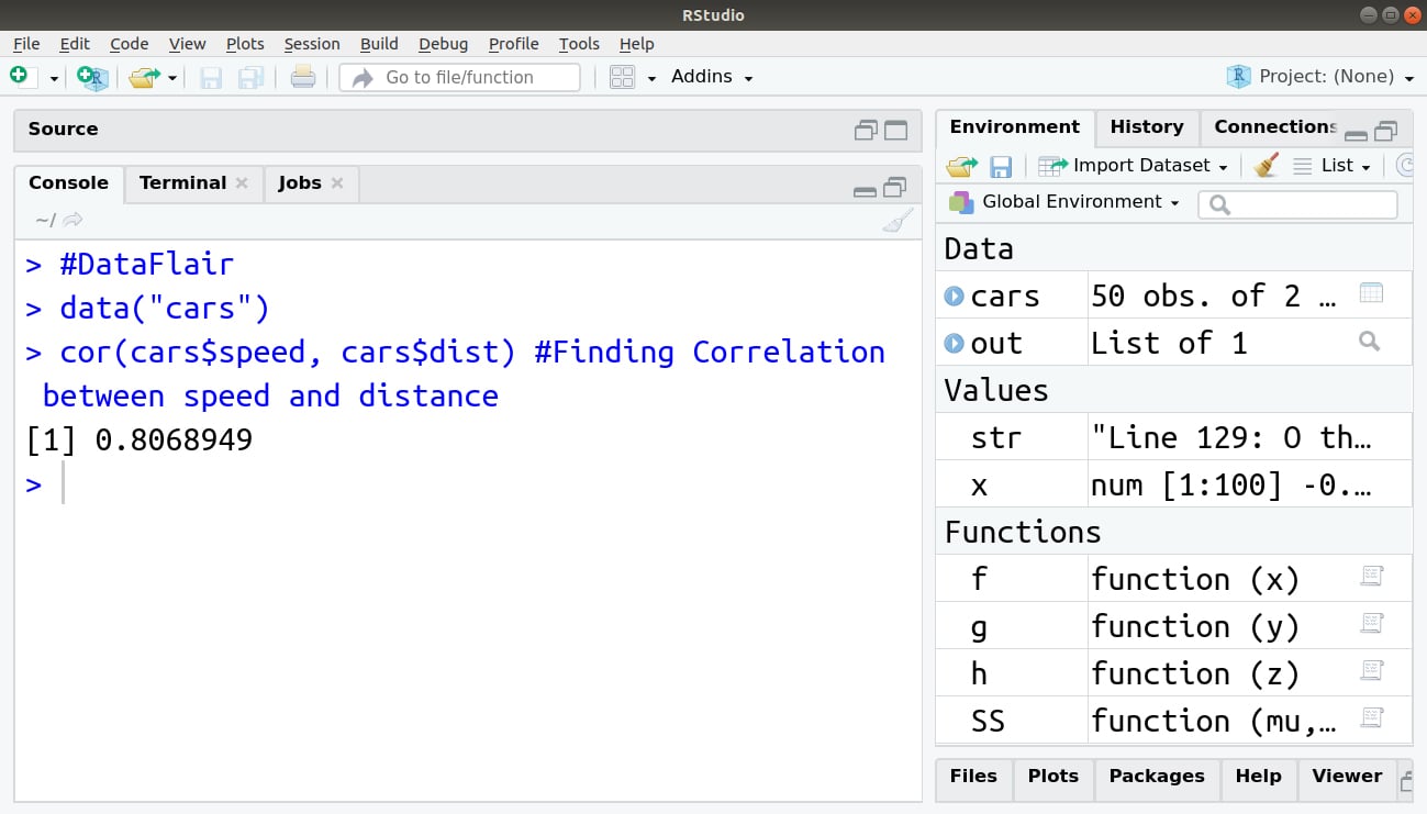
We can evaluate the correlation coefficient through the following data of the cars:
> #DataFlair
> data("cars")
> cor(cars$speed, cars$dist) #Finding Correlation between speed and distance
Output:
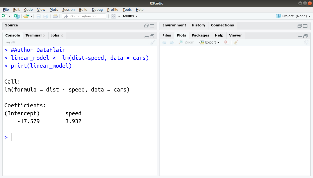
4. Building the Linear Model
In order to build our linear model, we will make use of the lm() function. We can write this function as follows:
> #Author DataFlair
> linear_model <- lm(dist~speed, data = cars)
> print(linear_model)
Output:
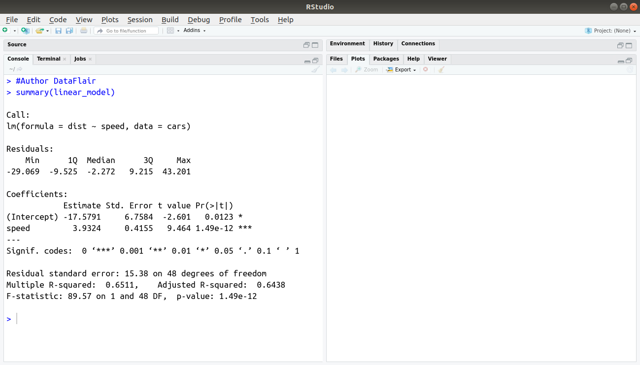
5. Diagnosing the Linear Model
After building our model, we can diagnose it by checking if it is statistically significant. In order to do so, we make use of the summary() function as follows:
> #Author DataFlair
> summary(linear_model)
Output:
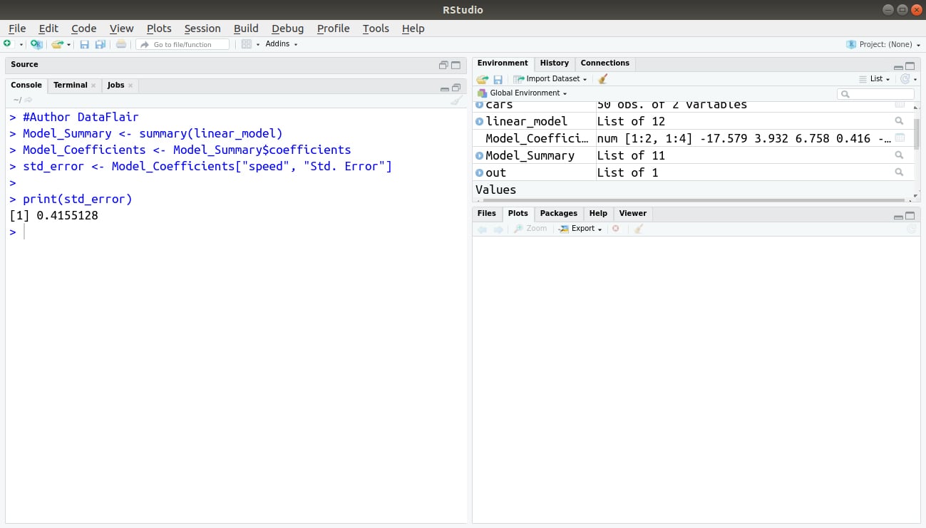
6. Calculating Standard Error and F – statistic
A Standard Error is the measurement of the standard deviation of the sample population from its mean.
![]()
Where MSE is the mean squared error. We can calculate the standard error in R as follows:
> #Author DataFlair
> Model_Summary <- summary(linear_model)
> Model_Coefficients <- Model_Summary$coefficients
> std_error <- Model_Coefficients["speed", "Std. Error"]
> print(std_error)
Output:
Another measure of the goodness of fit is F-statistic:
![]()
Where MSR is the mean squared regression:
> #Author DataFlair
> f_stat <- summary(linear_model)$fstatistic
> f_stat
Output:
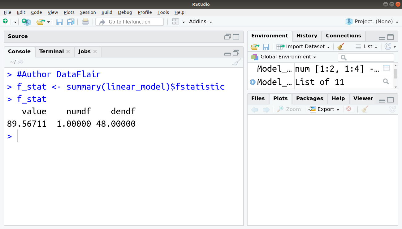
The F-statistic that we obtained for this model is 89.56711. The other two values of numdf and dendf can be used as parameters for calculating the p-value.
Use Case of Linear Regression
Linear Regression is used in various fields where a relationship between various instances (variables) is to be determined. Furthermore, with the determination of a relation, companies use linear regression to forecast future instances. Companies that have to increase their sales, use linear regression to identify the relationship between various factors and sale of their product.
For example – A company might want to analyse any relation between the use of their product by certain age-groups. Therefore, after the identification of the relationship, they can forecast if the customer of a particular age will buy their product. Linear Regression is also used to predict the housing prices, price of the tickets and several other areas where one instance might affect the another.
Summary
In this R Linear Regression tutorial, we discussed its core concept and working, in detail. We saw the least square estimation and checking model accuracy along with model building and implementing simple linear regression in R.
Next tutorial for you – R Nonlinear Regression
Still, if you have any doubt regarding R Linear Regression, ask in the comment section.
You give me 15 seconds I promise you best tutorials
Please share your happy experience on Google


