OLS Regression in R – 8 Simple Steps to Implement OLS Regression Model

Struggling to implement OLS regression In R? 

Forget all your troubles, you have landed on the most relevant page. This article is a complete guide of Ordinary Least Square (OLS) Regression Modeling. It will make you an expert in executing commands and implementing OLS regression in R programming.

What is OLS Regression in R?

OLS Regression in R programming is a type of statistical technique, that is used for modeling. It is also used for the analysis of linear relationships between a response variable. If the relationship between the two variables is linear, a straight line can be drawn to model their relationship. This will also fit accurately to our dataset.

The linear equation for a bivariate regression takes the following form:

y = mx + c

where, y = response(dependent) variable

m = gradient(slope)

x = predictor(independent) variable

c = the intercept

Wait! Have you checked – R Data Types

OLS in R – Linear Model Estimation using Ordinary Least Squares

1. Keywords

Models, regression

2. Usage

ols(formula, data, weights, subset, na.action=na.delete,

method=”qr”, model=FALSE,

x=FALSE, y=FALSE, se.fit=FALSE, linear.predictors=TRUE,

penalty=0, penalty.matrix, tol=1e-7, sigma,

var.penalty=c(‘simple’,’sandwich’), …)

3. Arguments

These are the arguments used in OLS in R programming:

• Formula – An S formula object, for example:

Y ~ rcs(x1,5)*lsp(x2,c(10,20))

• Data – It is the name of an S data frame containing all needed variables.
• Weights – We use it in the fitting process.
• Subset – It is an expression that defines a subset of the observations to use in the fit. The default is to use all observations.
• na.action – This specifies an S function to handle missing data.
• Method – This specifies a particular fitting method, or “model.frame”.
• Model – The default is FALSE. It is set to TRUE. This attribute returns the model frame in the form of an element that is able to fit the object.
• X – The default is FALSE. It is set to TRUE to return the expanded design matrix as element x of the returned fit object. First, set both x=TRUE, if you are going to use the residuals function.
• Y – The default is FALSE.  It is set to TRUE to return the vector of response values as element y of the fit.
• Se.fit – The default is FALSE. It is set to TRUE that computes the estimated standard errors of the estimate of Xβ. And, also store them in element se.fit of the fit.
• Linear.predictors – It is set FALSE as default. It is used to cause predicted values not to be stored.
• Penalty penalty.matrix – see lrm
• Tol – Tolerance for information matrix singularity.
• Sigma – If sigma is given, then we can use it as the actual root mean squared error parameter for the model. We also use sigma as an estimation from the data that consists of the usual formulas.
• Var.penalty – It is the type of variance-covariance matrix that is to be stored in the var component of the fit when penalization is used.
• p. – We pass the arguments to lm.wfit or lm.fit.

Do you know – How to Create & Access R Matrix?

OLS Data Analysis: Descriptive Stats

Several built-in commands for describing data has been present in R.

• We use list() command to get the output of all elements of an object.
• The summary() command is used to describe all variables contained within a data frame.
• We use summary() command with individual variables.
• Simple plots can also provide familiarity with the data.
• The hist() command produces a histogram for any given data values.
• We use the plot() command which produces both univariate and bivariate plots for any given objects.

1. Other Useful Commands:

• sum
• min
• max
• mean
• median
• var
• sd
• cor
• range
• Summary

OLS Regression Commands for Data Analysis

These are useful OLS regression commands for data analysis:

• lm – Linear Model

• lme – Mixed effects

• glm – General lm

• Multinomial – Multinomial Logit

• Optim – General Optimizer

You must definitely check the Generalized Linear Regression in R

How to Implement OLS Regression in R

To implement OLS in R, we will use the lm command that performs linear modeling. The dataset that we will be using is the UCI Boston Housing Prices that are openly available.

For the implementation of OLS regression in R, we use – Data (CSV)

So, let’s start with the steps with our first R linear regression model.

Step 1:  First, we import the important library that we will be using in our code.

> library(caTools)

Output:

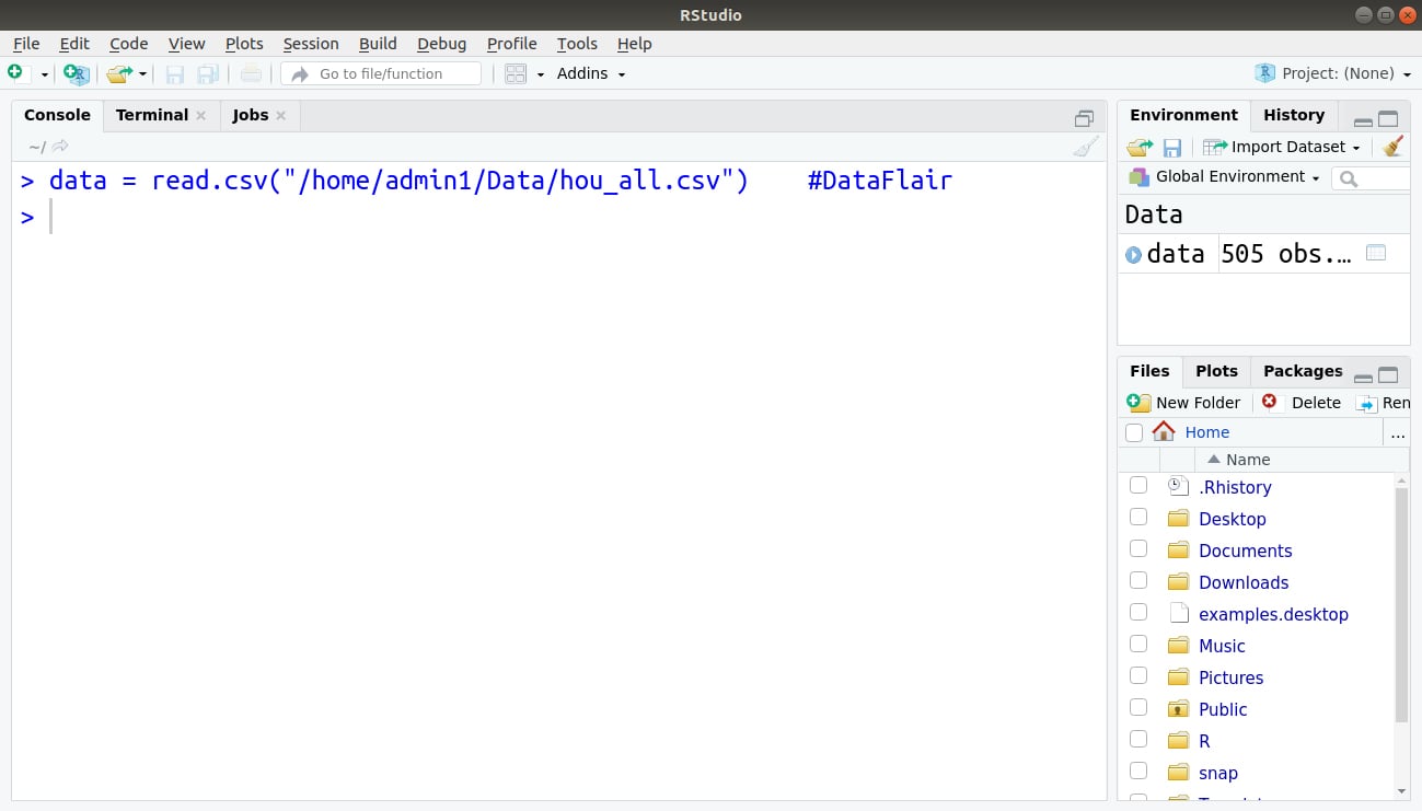
Step 2: Now, we read our data that is present in the .csv format (CSV stands for Comma Separated Values).

> data = read.csv("/home/admin1/Desktop/Data/hou_all.csv")

Output:

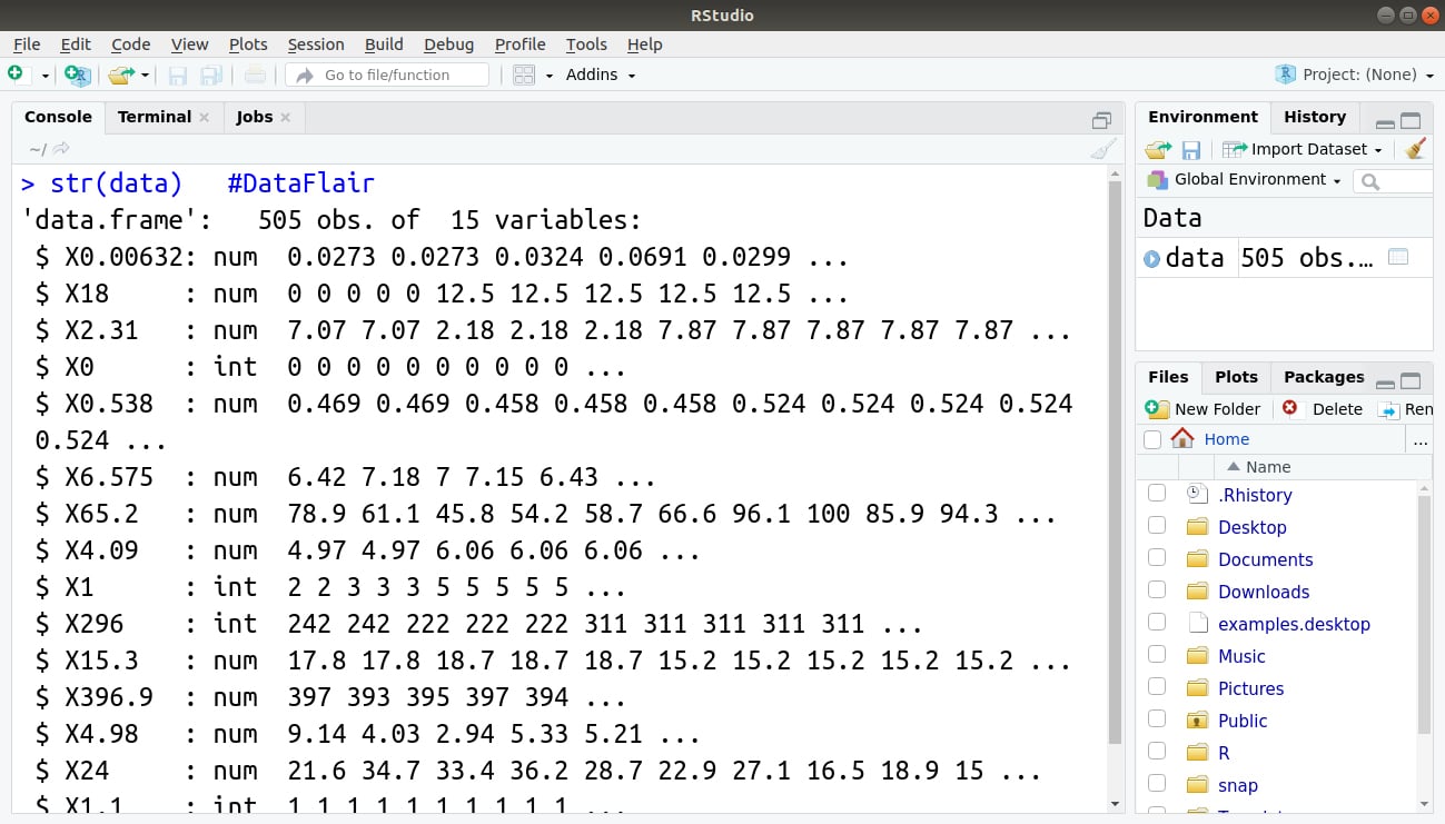
Step 3: Now, we will display the compact structure of our data and its variables with the help of str() function.

> str(data)

Output:

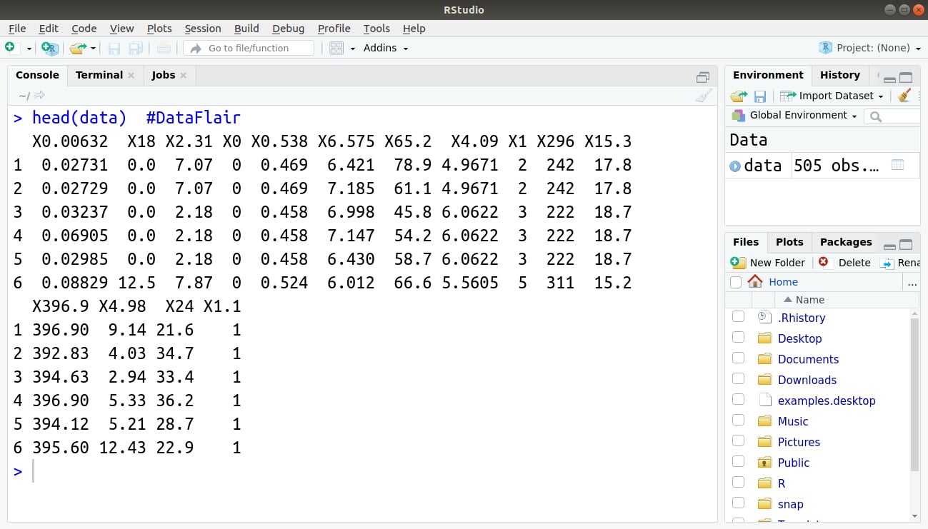
Step 4: Then to get a brief idea about our data, we will output the first 6 data values using the head() function.

> head(data)

Output:

Step 5: Now, in order to have an understanding of the various statistical features of our labels like mean, median, 1st Quartile value etc., we use the summary() function.

> summary(data)

Output:

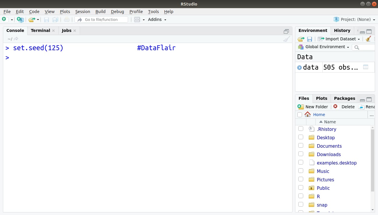
Step 6: Now, we will take our first step towards building our linear model. Firstly, we initiate the set.seed() function with the value of 125. In R, set.seed() allows you to randomly generate numbers for performing simulation and modeling.

> set.seed(125)

Output:

Step 7: The next important step is to divide our data into training data and test data. We set the percentage of data division to 75%, meaning that 75% of our data will be training data and the rest 25% will be the test data.

> data_split = sample.split(data, SplitRatio = 0.75)
> train <- subset(data, data_split == TRUE)
> test <-subset(data, data_split == FALSE)

Output:

Step 8: Now that our data has been split into training and test set, we implement our linear modeling model as follows:

model <- lm(X1.1 ~ X0.00632 + X6.575 + X15.3 + X24, data = train) #DataFlair

Output:

Lastly, we display the summary of our model using the same summary() function that we had implemented above.

> summary(model)

Output:

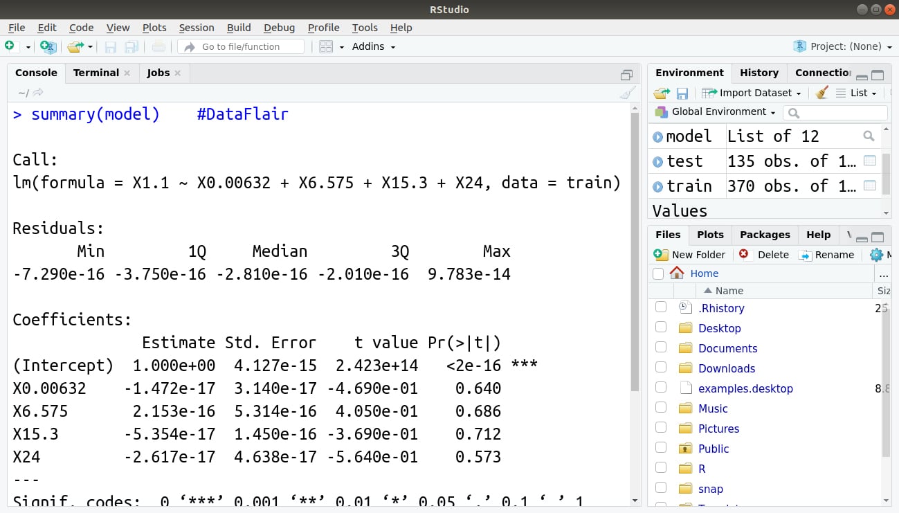
And, that’s it! You have implemented your first OLS regression model in R using linear modeling!

OLS Diagnostics in R

• Post-estimation diagnostics are key to data analysis.

• We can use diagnostics which allows us the opportunity to show off some of the R’s graphs. What else could be driving our driving our data?

-Outlier: Basically, it is an unusual observation.

-Leverage: It has the ability to change the slope of the regression line.

-Influence: The combined impact of strong leverage and outlier status.

It’s the right time to uncover the Logistic Regression in R

Summary

We have seen how OLS regression in R using ordinary least squares exist. Also, we have learned its usage as well as its command. Moreover, we have studied diagnostic in R which helps in showing graph. Now, you are an expert in OLS regression in R with knowledge of every command.

If you have any suggestion or feedback, please comment below.