R Nonlinear Regression Analysis – All-inclusive Tutorial for Newbies!
Job-ready Online Courses: Click, Learn, Succeed, Start Now!
Previously, we learned about R linear regression, now, it’s the turn for nonlinear regression in R programming. We will study about logistic regression with its types and multivariate logit() function in detail. We will also explore the transformation of nonlinear model into linear model, generalized additive models, self-starting functions and lastly, applications of logistic regression.
R Nonlinear Regression Analysis
R Nonlinear Regression and Generalized Linear Models:
Regression is nonlinear when at least one of its parameters appears nonlinearly. It commonly sorts and analyzes data of various industries like retail and banking sectors. It also helps to draw conclusions and predict future trends on the basis of the user’s activities on the internet.
The nonlinear regression analysis in R is the process of building a nonlinear function. On the basis of independent variables, this process predicts the outcome of a dependent variable with the help of model parameters that depend on the degree of relationship among variables.
Generalized linear models (GLMs) calculates nonlinear regression when the variance in sample data is not constant or when errors are not normally distributed.
A generalized linear model commonly applies to the following types of regressions when:
- Count data is expressed as proportions (e.g. logistic regressions).
- Count data is not expressed as proportions (e.g. log-linear models of counts).
- We have binary response variables (e.g. “yes/no”, “day/night”, “sleep/awake”, buy/not buy).
- Data is showing a constant coefficient of variation (e.g. time data with gamma errors).
Learn about the concept of Generalized Linear Models in R Programming in detail
Logistic Regression in R
In statistics, logistic regression is one of the most commonly used forms of nonlinear regression. It is used to estimate the probability of an event based on one or more independent variables. Logistic regression identifies the relationships between the enumerated variables and independent variables using the probability theory.
A variable is said to be enumerated if it can possess only one value from a given set of values.
Logistic Regression Models are generally used in cases when the rate of growth does not remain constant over a period of time. For example -when a new technology is introduced in the market, firstly its demand increases at a faster rate but then gradually slows down.
Logistic Regression Types:
- Multivariate Logistic Regression – Here logistic regression includes more than one independent variable. Multivariate logistic regression is commonly used in the fields of medical and social science. It is also used to make electoral assumptions such as the percentage of voting in a particular area; the ratio of voters in terms of sex, age, annual income, and residential location; and the chances of a particular candidate to win or lose from that area. This analysis helps to predict the level of the failure or success of a proposed system, product, or process.
- Multinomial Logistic Regression – Here set of possible values are more than two. It is used to estimate the value of an enumerated variable when the value of the variable depends on the values of two or more variables.
Logistic regression is defined using logit() function:
f(x) = logit(x) = log(x/(1-x))
Suppose p(x) represents the probability of the occurrence of an event, such as diabetes and on the basis of an independent variable, such as age of a person. The probability p(x) will be given as follows:
P(x)=exp(β0+ β1x1 )/(1+ exp(β0+ β1x1)))
Here β is a regression coefficient.
On taking the logit of the above equation, we get:
logit(P(x))=log(1/(1-P(x)))
On solving the above equation, we get:
logit(P(x))=β0+ β1x1
The logistic function that is represented by an S-shaped curve is known as the Sigmoid Function.
When a new technology comes in the market, usually its demand increases at a fast rate in the first few months and then gradually slows down over a period of time. This is an example of logistic regression. Logistic Regression Models are generally used in cases where the rate of growth does not remain constant over a period of time.
Multivariate logit() Function
In case of multiple predictor variables, following equation represent logistic function:
p = exp(β0+ β1x1+ β2x2+—– βnxn)/(1+exp(β0+ β1x1+ β2x2+…+βnxn))
Here, p is the expected probability; x1,x2,x3,…,xn are independent variables; and β0, β1, β2,…βn are the regression coefficients.
Estimating β Coefficients manually is an error-prone and time-consuming process, as it involves lots of complex and lengthy calculations. Therefore, such estimates are generally made by using sophisticated statistical software.
β coefficients need to be calculated in statistical analysis. For this, follow the below steps:
- Firstly, you need to calculate the logarithmic value of the probability function.
- Now, calculate the partial derivatives with respect to each β coefficient. For n number of unknown β coefficients, there will be n equations.
- For n unknown β coefficients, you need to set n equations.
- Finally, to get the values of the β coefficients, you can solve the n equations for n unknown β coefficients.
Interaction is a relationship among three or more variables to specify the simultaneous effect of two or more interacting variables on a dependent variable. We can calculate the logistic regression with interacting variables, that is three or more variables in relation where two or more independent variables affect the dependent variable.
In logistic regression, an enumerated variable can have an order but it cannot have magnitude. This makes arrays unsuitable for storing enumerated variables because arrays possess both order and magnitude. Thus, enumerated variables are stored by using dummy or indicator variables. These dummy or indicator variables can have two values: 0 or 1.
After developing a Logistic Regression Model, you have to check its accuracy for predictions. Adequacy Checking Techniques are explained below:
- Residual Deviance – High residual variation refers to insufficient Logistic Regression Model. The ideal value of residual variance Logistic Regression Model is 0.
- Parsimony – Logistic Regression Models with less number of explanatory variables are more reliable than models with a large number of explanatory variables and can be more useful also.
- Classification Accuracy – It refers to the process of setting the threshold probability for a response variable on the basis of explanatory variables. It helps to interpret the result of a Logistic Regression Model easily.
- Prediction Accuracy – To check the accuracy of predictions for the Logistic Regression Model, cross-validation is used which is repeated several times to improve the prediction accuracy of the Logistic Regression Model.
You must definitely learn about the Implementation of Logistic Regression in R
Applications of Logistic Regression
Logistic regression is the most commonly used form of regression analysis in real life. As a result, they are quite useful for classifying new cases into one of the two outcome categories.
Let’s check some of the applications:
- Loan Acceptance – By using logistic regression, on the basis of the customer’s previous behaviour, organizations which provide banks or loan can determine whether the customer would accept an offered loan or not. Various explanatory variables include the age of customer, experience, the income of the customer, family size of customer, CCAvg, Mortgage, etc.
- German Credit Data – The German credit dataset was obtained from the UCI (the University of California at Irwin) Machine Learning Repository (Asuncion and Newman, 2007). The dataset, which contains attributes and outcomes of 1,000 loan applications, was provided in 1994 by Dr Hans Hofmann of the institute,für Statistik und Ökonometrie at the University of Hamburg. It also served as an important test dataset for several credits coring algorithms. The logistic expression is used to estimate the probability of default, using continuous variables (duration, amount, instalment, age) and categorical variables (loan history, purpose, foreign, rent) as explanatory variables.
- Delayed Airplanes – Logistic regression analysis can also predict a possible delay in airplane timing. Explanatory variables include different arrival airports, different departure airports, carriers, weather conditions, the day of the week and a categorical variable for different hours of departure.
Line Estimation using MLE
Regression lines for models are generated on the basis of the parameter values that appear in the regression model. So first you need to estimate the parameters for the regression model. Parameter estimation is used to improve the accuracy of linear and nonlinear statistical models.
The process of estimating the parameters of a regression model is called Maximum Likelihood Estimation (MLE).
We can estimate the parameters in any of the following ways:
- You can specify the model parameters with certain conditions, such as the resistance of a mechanical engine and inertia.
- You can manipulate input and output test data, such as the rate of the influx of current and output of the mechanical engine in round per minute (rpm).
- On different values of a variable, you can perform a number of measurements for a function.
The presence of bias while collecting data for parameter estimation might lead to uneven and misleading results. Bias can occur while selecting the sample or collecting the data.
Don’t forget to check the R Statistics Tutorial
Transformation of a Nonlinear Model into a Linear Model
Linear least square method fits data points of a model in a straight line. However, in many cases, data points form a curve.
Nonlinear models are sometimes fitted into linear models by using certain techniques as linear models are easy to use. Consider the following equation which is a nonlinear equation for exponential growth rate:
y=cebxu
Here b is the growth rate while u is the random error term and c is a constant.
We can plot a graph of the above equation by using the linear regression method. Implement the following steps to transform the above nonlinear equation into a linear equation, as follows:
- On taking these base logarithm of the equation, you get the result as In(y)-In(c)+bx+In(u).
- Now, if you substitute Y for In(y), C for In(c), and U for In(u), you will get the following result: Y-A+bx+U.
Other R Nonlinear Regression Models
There are several models for specifying the relationship between y and x and estimate the parameters and standard errors of parameters of a specific nonlinear equation from data.
Some of the most frequently appearing nonlinear regression models are:
a) Michaelis-Menten
y=ax/(1+bx)
b) 2-parameter asymptotic exponential
y=a(1−e-bx)
c) 3-parameter asymptotic exponential
y=a−be−cx
Below are few S-shaped Functions:
d) 2-parameter logistic
y=( ea+bx)/(1+ea+bx)
e) 3-paramerter logistic
y=a/(1+be−cx)
f) 3-parameter asymptotic exponential
y=a/(1+be−cx)
g) Weibull
y=a- be-(cx2)
Below are few Humped Curves:
h) Ricker curve
y=axe−bx
i) First-order compartment
y=kexp(−exp(a)x)−exp(−exp(b)x)
j) Bell-shaped
y=a exp(−|bx|2)
k) Biexponential
y=aebx −ce−dx
The accuracy of a statistical interpretation largely depends on the correctness of the statistical model on which it depends.
The following are the most common statistical models:
- Fully Parametric – In this model, assumptions are on the basis of the number of parameters known.
- Non-Parametric – In this model, assumptions are on the basis of the features of the available data. These models do not use parameters to describe the process of generating data.
- Semi Parametric – In this model, both parametric and nonparametric approaches describe the process of data generation. These models use parameters as well as the main features of the data to derive conclusions.
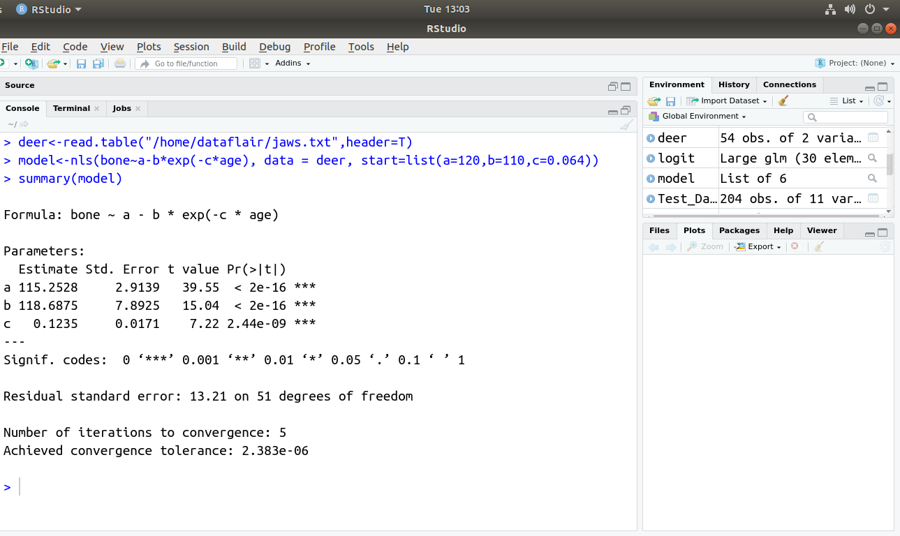
An example of nonlinear regression: This example is based on the relationship between jaw bone length and age in deers.
- Reading the dataset from jaws.txt file; Path of the file acts as an argument.
deer<-read.table("c:\\temp\\jaws.txt",header=T)You can download the dataset from here – jaws file
- Fitting the model – Nonlinear equation is an argument in nls() command with starting values of a, b and c parameters. The result goes in the model object.
model<-nls(bone~a-b*exp(-c*age),start=list(a=120,b=110,c=0.064))
- Displaying information about a model object using the summary() command. The model object is an argument to the summary() command as shown below:
summary(model)
Output:
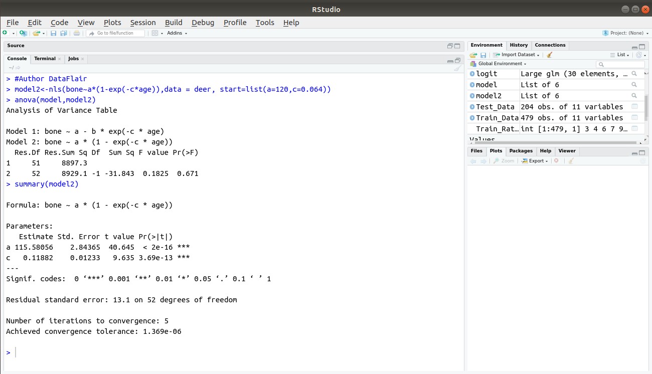
- Fitting a simpler model
y=a (1−e−cx)
- Applying nls() command to the new model for the modified regression model. The result goes in the model2 object.
model2<-nls(bone~a*(1-exp(-c*age)),start=list(a=120,c=0.064))
Comparing the models as below – Use anova() command to compare result objectsmodel1 and model2. These objects then act as arguments to anova() command.
anova(model,model2)
Viewing the components of the New Model2 as below:
summary(model2)
Output:
Wait! Have you completed the R Graphical Models Tutorial
Generalized Additive Models (GAM)
Sometimes we can see that the relationship between y and x is nonlinear but we don’t have any theory or any mechanistic model to suggest a particular functional form (mathematical equation) to describe the relationship. In such circumstances, Generalized Additive Models (GAMs) are particularly useful because they fit a nonparametric curve to the data without requiring us to specify any particular mathematical model to describe the nonlinearity.
GAMs are useful because they allow you to identify the relationship between y and x without choosing a particular parametric form. Generalized additive models implemented in R by the function gam() command.
The gam() command has many of the attributes of both glm() and lm(), and we can modify the output using update() command. You can use all of the familiar methods such as print, plot, summary, anova, predict, and fitted after a GAM has been fitted to data. The gam function is available in the mgcv library.
Self-Starting Functions
In nonlinear regression analysis, the nonlinear least-squares method becomes insufficient because the initial guesses by users for the starting parameter values may be wrong. The simplest solution is to use R’s self-starting models.
Self-starting models work out the starting values automatically and nonlinear regression analysis makes use of this to overcome the chances of the initial guesses, which the user tends to make, being wrong.
Some of the most frequently used self-starting functions are:
1. Michaelis-Menten Model(SSmicmen)
R has a self-starting version called SSmicmen that is as follows:
y=ax/(b+x)
Here, a and b are two parameters, indicating the asymptotic value of y and x (value at which we get half of the maximum response a/2) respectively.
2. Asymptotic Regression Model (SSasymp)
Below gives the self-starting version of the asymptotic regression model.
3 parameter asymptotic exponential equation can be as:
y=a−be−cx
Here, a is a horizontal asymptote, b=a-R0 where R0 is the intercept (response when x is 0), and c is rate constant.
3. Four Parameter Logistic Model (SSfpl)
y=A+(B-A)/(1+e(D-x)/c)
Here, A is horizontal asymptote on left (for low values of x), B is horizontal asymptote on right (for large values of x), D is the value of x at the point of inflection of the curve, and c is a numeric scale parameter on the X-axis. It gives the self-starting version of four-parameter logistic regression.
4. Self-Starting First-Order Compartment Function (SSfol)
This function is given as follows:
y=k exp(−exp(a)x)−exp(−exp(b)x)
Here, k=Dose*exp(a+b−c)/(exp(b)- exp(a)) and Dose is a vector of identical values provided to the fit. It gives the self-starting version of first-order compartment function.
5. Self-Starting Weibull Growth Function (SSweibull)
R’s parameterization of the Weibull growth function is as follows:
Asym-Drop*exp(-exp(lrc)*x^pwr)
It gives the self-starting version of Weibull growth function.
Here, Asym is the horizontal asymptote on the right
Drop is the difference between the asymptote and the intercept (the value of y at x=0)
lrc is the natural logarithm of the rate constant
pwr is the power to which x is raised.
Summary
We learned about the complete concept of nonlinear regression analysis in R programming. We understood the R logistic regression with its applications, line estimation using MLE, R nonlinear regression models and self-starting functions.
Now, we will learn to Create Decision Trees in R Programming
If you have any queries regarding R nonlinear regression, ask in the comment section.
We work very hard to provide you quality material
Could you take 15 seconds and share your happy experience on Google


HOW TO DO MULTIPLE NONLINEAR REGRESSION IN R (5 INDEPENDENT VARIABLE AND ONE DEPENDENT VARIABLE)
Thank you very much for detail explanations about the nonlinear regression and estimation methods using R software.
I have some questions, The first is that, does the gam() function in R or general additive estimation method of non-linear regression model doesn`t assume the distributions of error terms? if so the extension VGAM for multivariate nonlinear regression is available in R?
Finally, can I apply lm() function in R to estimate the coefficients of transformable linear models?
Thank you.
> y=a (1−e−cx)
Error: unexpected input in “y=a (1−”
respected author please check this error
In case, if, it’s simply an example, please, put # or just say it’s an example. so, the reader can ignore the coming error in the console
and please reply to comments so we can expand our knowledge
Thanks a lot. Can I get more tutorial in R, I think have fall in love with the simplicity of it