Statistics and R – Clear up your Stats problems with R Programming!
FREE Online Courses: Click, Learn, Succeed, Start Now!
“Statistics can be made to prove anything – Even the truth”
Have you ever solved any statistics problem in just a few minutes? I bet you never did so. In fact, even I was unable to solve statistics problems until I got to know about R programming. Yes! R is the ultimate solution to every statistics problem and DataFlair is the way to master R programming. Today, I am going to clear every doubt of yours related to Statistics and R. So, follow the blog and learn statistics with R.
Introduction to Statistics for R
R Statistics concerns data; their collection, analysis, and interpretation. It has the following two types:
- Descriptive statistics
It is about providing a description of the data. It deals with the quantitative description of data through numerical representations or graphs.
Example: Normal Distribution, Central Tendency, Kurtosis, etc. are some of the statistical techniques in Descriptive Statistics.
- Inferential statistics
It is a step ahead of former. In inferential statistics, we draw conclusions or ‘inferences’ from our dataset. Also, a conclusion is drawn about the larger population from a data of a much smaller sample.
Example: Central Limit Theorem, Hypothesis Testing, ANOVA are some of the inferential statistics techniques.
Types of Data in Statistics
Whenever we are working with statistics. It’s very important to recognize the different types of data:
- Numerical (discrete and continuous)
- Categorical
- Ordinal
Data is nothing but information that is gathered as a result of a survey.
Data can either be numerical or categorical in nature.
1. Numerical Data
It contains data that can be measured. A person’s height, weight, IQ, or blood pressure are examples of Numerical Data.
Numerical Data is again of two types –
- Discrete
- Continuous.
a. Discrete data – It represents items that can be counted. Basically, they take on possible values that can be listed out. The list of possible values may be fixed or it may go to infinity.
b. Continuous data – It represents measurements. Also, their possible values cannot be counted. Although, it can only be described using intervals on the real number line.
Don’t forget to check the complete guide on R predictive and Descriptive analytics
2. Categorical Data
Categorical Data is used to represent characteristics that are present in the data such as a person’s gender, marital status, hometown.
For example, in a given group of males and females, males can be represented as 0 and females can be represented as 1. Therefore, we have two classes of distinct characteristics.
There is one more data called Ordinal Data. Let’s begin to learn this –
3. Ordinal data
In this form of data, the variables have an ordered category which is natural and the distance between these variables is not known. Ordinal Data is similar to categorical data with the only difference that the data is ordered.
For example, Rating a restaurant on a scale of 0 to 4 gives us ordinal data.
They are often treated as categorical. We have to order the groups whenever it is required to create graphs and charts.
Must-read blog in R statistics – The concept of Chi-Square Test
Distance Measures (Similarity, dissimilarity, correlation)
We consider it as mathematical approaches. Also, it helps us to measure the distance between the objects. Also, we use computing distance to compare the objects. Now, we can conclude three different standpoints on the basis of comparison such as:
- Similarity- A measure that ranges from 0 to 1 [0, 1]
- Dissimilarity- It is measured that ranges from 0 to INF [0, Infinity]
- Correlation- It is measures that ranges from +1 to -1 [+1, -1]
Now, to become a pro in statistics for R, you can’t miss learning the concept of correlation. So, let me tell you what exactly correlation is –
What is Correlation?
Correlation is a statistical technique for measuring the relationship between the two variables. It is of three types- Positive Correlation, Negative Correlation, and Zero Correlation.
In a positive correlation, both variables increase and decrease together. Whereas, in a negative correlation, one variable increases and the other decreases. And, finally, in the case of zero correlation, there is no relation between the variables.
Correlation is represented by ‘r’ and ‘r’ can range from -1 to +1.
- If r is close to 0, it means there is no relationship between the objects.
- When r is positive, it means that the value of one variable increases, the value of other variable increases.
- If r is negative means the value of one variable increases, the value of other variable decreases.
A Gentle Reminder!!! Don’t miss the opportunity to learn survival analysis wit experts
What is Pearson’s Correlation Coefficient?
Pearson Correlation is used for measuring the linear relationship between the variables X and Y. The value of this coefficient is between +1 and -1. Pearson’s correlation coefficient is the covariance of the two variables divided by the product of their standard deviations.
For example, age and blood pressure.
Values of Pearson’s correlation coefficient
The data in the continuous interval has a Pearson Correlation Coefficient ranging from -0.4 to +0.4
Graphically correlations look like:
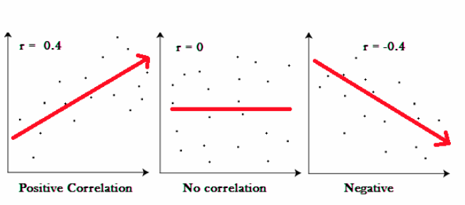
If r = -0.4, data lie on a perfectly straight line with a negative slope.
For r = +0.4, data lie on a perfectly straight line with a positive slope.
When r = 0, no linear relationship between the variables.
Positive correlation – In this, both variables increase or decrease together.
Negative correlation – In this correlation as one variable increases, so other decreases.
If you have any doubt regarding R concepts, reach out to our Free R Tutorials Series. Here you will find each and every concept related to R for FREE.
Formulas and Methods to Calculate Distance Measure
Now we will see different formulas that are used for calculating distance measure in Statistics for R –
- Euclidean distance
- Taxicab or Manhattan distance
- Minkowski
- Cosine similarity
- Mahalanobis distance
- Pearson’s Correlation Coefficient (discussed above)
a. Euclidean Distance
It is a classical method of computing the distance between the two points. These two points – A and B are said to be in the Euclidean Space.
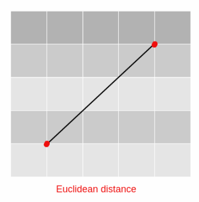
It can be used to measure distance in either a plane or a 3-D space. You can derive the Euclidean distance using Pythagoras Theorem.
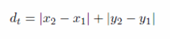
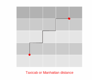
b.Taxicab or Manhattan Distance
This is similar to Euclidean Distance with only a single difference. The distance is calculated through traversing. Furthermore, the traversing is performed in vertical & horizontal line in the grid-based system.
Geographically we use it to measure the separation between building blocks in the city.
For Example:
Manhattan distance used to calculate a distance between two points. Geographically we use it to separate by the building blocks in the city.
Keywords
visualization, manhattan
Want to master R Programming? You need to explore R data analysis tools!
c. Minkowski
This distance is a metric on Euclidean space. We can also consider it as s a generalization of Euclidean and Manhattan distance.
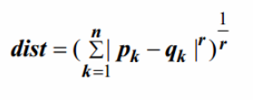
Where r is a parameter.
- When r =1
It tends to compute Manhattan distance.
- When r =2
It tends to compute Euclidean distance.
- When r =∞
It tends to compute Supremum.
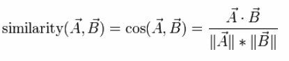
d. Cosine Similarity
It is a measure that calculates the cosine of the angle between two vectors. Basically, this metric is a measurement of orientation and not size.
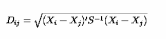
e. Mahalanobis distance
Mahalanobis distance is a metric of measurement of the distance between two points in multivariate space. In cases of uncorrelated variables, the Euclidean Distance is equal to Mahalanobis Distance. However, if two or more variables are uncorrelated, then the axes are no longer at right angles. Therefore, plotting them in a regular 3D space becomes a problem.
The Mahalanobis distance rectifies this problem and facilitates measurement, even between uncorrelated points in a multi-variable space. The formula for MD is as follows –
Keywords
Mahalanobis distance
So, this was all about the statistics and R concepts. Hope you understand all the formulas and methods. Still, if you face any trouble, ask in the comment section. We will definitely reply.
You should check what’s trending on DataFlair – Latest R project for freshers
Your 15 seconds will encourage us to work even harder
Please share your happy experience on Google


good evening I would like to ask you can I use R for the replenishment of daily rains by adding packages like python and anaconda and if there is another program to highlight the gaps
thank you