R Clustering Tutorial – R Cluster Analysis
Placement-ready Courses: Enroll Now, Thank us Later!
1. Objective
In this tutorial, we will discuss R Clustering in detail. Also, we will look at Clustering in R goal, R clustering types, usages, applications of R clustering and many more. Moreover, we will also cover common types of algorithms based on clustering and k means Clustering in R. Along with this, we use images, graphs for algorithms for clear and better understanding.
So, let’s start the R Clustering tutorial.
R Clustering Tutorial – R Cluster Analysis
2. What is R Cluster Analysis?
First of all, let us see what is R clustering
We can consider R clustering as the most important unsupervised learning problem. Therefore, for every other problem of this kind, it has to deal with finding a structure in a collection of unlabeled data.
“It is the process of organizing objects into groups whose members are similar in some way”.
R clustering is a collection of objects. Which are “similar” to them? Also, “dissimilar” to the objects belonging to other clusters.
Before learning about R clustering, let us revise our concepts of Introduction to R programming language.
3. R Clustering – Goals
To determine the intrinsic grouping in a set of unlabeled data. Although, problem is that how to decide what forms a good clustering? Moreover, It is being shown that there is no absolute “best” criterion. So it would be independent of the final aim of the clustering.
4. Types of R Clustering
i. Hard Clustering
In this, each data point either belongs to a cluster completely or not.
ii. Soft Clustering
In this, we assign a probability of the data point. Although, instead of putting each data point into a separate cluster.
5. Requirements for R clustering
The main requirements that a clustering algorithm should meet are:
- Scalability;
- It must deal with different types of attributes;
- Clustering discover clusters with arbitrary shape;
- It has the ability to deal with noise and outliers;
- High dimensionality;
- Interpretability and usability.
6. Applications of R Clustering
We can apply it in many fields:
- Marketing: It helps in finding the groups of customers with similar behavior. Thus, provides a large database of customer data. Also, it contains the properties and past buying records.
- Biology: Clustering helps in the classification of plants and animals given their features.
- Libraries: Helps in book order.
- Insurance: clustering needs in identifying groups of motor insurance policyholders. Which is having a high average claim cost? identifying frauds.
- City-planning: It helps in identifying groups of houses. Although, according to their house type, value and geographical location.
- Earthquake studies: It observed earthquake epicenters to identify dangerous zones.
7. Problems with R Clustering
There are some problems with clustering. We will discuss among them:
- We face problem in addressing the requirements because of Current clustering techniques.
- Time complexity is the main reason that makes the problem.
- We can interpret the result of the clustering algorithm in different ways.
8. Types of R Clustering Algorithm
Let’s look at some of them in detail:
i. Distribution models
These are based on the notion of how probable is it that all data points in the cluster belong to the same distribution. These models often suffer from overfitting.
For Example:
Model-based clustering: It is being used on a heuristic approach to constructing clusters. it assumes a data model. Also, we can apply an EM algorithm. That’s need to find the most likely model components and the number of clusters.
ii. Connectivity models
It is based on the notion. The data points closer in data space exhibit more similarity to each other.
These models can follow two approaches:
- We first start with classifying all data points into separate clusters. Then aggregating them as the distance decreases.
- All data points are classified as a single cluster. Then partitioned as the distance increases. Also, the choice of the distance function is subjective. These models are very easy to interpret. But lack scalability for handling big data sets.
For Example:
Hierarchical clustering: It helps in creating a hierarchy of clusters. Then presents the hierarchy in a dendrogram. In this method, he does not need any number of clusters to be specified at the beginning.
iii. Density Models
It helps in searching the data space for areas of varied density of data points in the data space. It isolates different density regions. Also, assigns the data points within these regions in the same cluster.
For Example:
Density-based R Clustering: In regards to the density measurement it creates clusters. In this method, we have known that cluster has a higher density than the rest of the dataset. Density in data space is the measure.
iv. Centroid models
These are iterative clustering algorithms. In this, the notion of similarity is derived by the closeness of a data point to the centroid of the clusters.
For Example:
K-means clustering: It is also referred to as flat clustering. Also, it requires the number of clusters as an input. But, its performance is faster than hierarchical clustering. Distance from the mean value of each observation/cluster is the measure.
Now I will be taking you through three of the most popular algorithms for R Clustering in detail:
- K Means clustering:
- DBSCAN clustering, and
- Hierarchical clustering.
a. K-means Clustering in R
The most common partitioning method is the K-means cluster analysis. It is an unsupervised learning algorithm. it tries to cluster data based on their similarity. Also, we have specified the number of clusters. And we want the data must be group into same clusters. The algorithm assigns each observation to a cluster. Also, finds the centroid of each cluster.
The K-means algorithm:
- Selects K centroids (K rows chosen at random)
- Then we have to assign each data point to its closest centroid.
- Moreover, recalculates the centroids as the average of all data points in a cluster.
- Assigns data points to their closest centroids.
- Moreover, we have to continue steps 3 and 4 until the observations are not reassigned
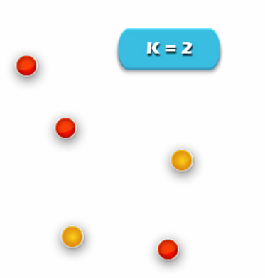
Image.2 Clustering in R – R Cluster Analysis
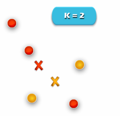
Image.3 R Clustering – R Cluster Analysis
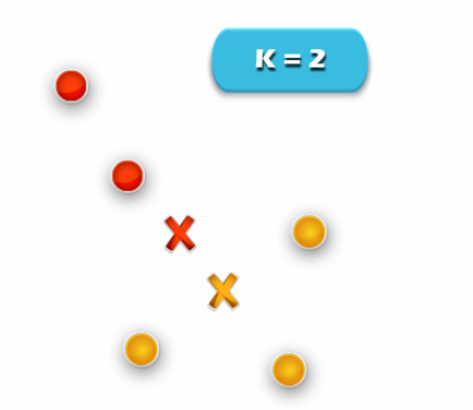
Image.4 R Clustering – R Cluster Analysis
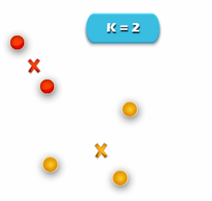
Image.6 R Clustering – R Cluster Analysis
This algorithm works in these 5 steps :
1. Specify the desired number of clusters K: Let us choose k=2 for these 5 data points in 2D space.
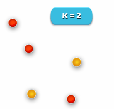
Image.5 Clustering in R – R Cluster Analysis
2. Assign each data point to a cluster:
Let’s assign three points in cluster 1 shown using red color and two points in cluster 2 shown using yellow color.
3. Compute cluster centroids:
The centroid of data points in the red cluster is shown using the red cross. Also, those in a yellow cluster using a yellow cross.
4. Re-assign each point to the closest cluster centroid:
The data point at the bottom is assigned to the red cluster. If even though it’s closer to the centroid of the yellow cluster. Thus, we assign that data point into a yellow cluster.
5. Re-compute cluster centroids: Now, re-computing the centroids for both the clusters.
Repeat steps 4 and 5 until no improvements are possible. We’ll repeat the 4th and 5th steps until we’ll reach global optima. When there will be no further switching of data points. Then it will mark the termination of the algorithm if not mentioned.
b. DBSCAN R Clustering
It was introduced in Ester et al. 1996. That can be used to identify clusters of any shape in a dataset containing noise and outliers. Although, it is a technique that allows partitioning data into groups with similar characteristics. But it does need specifying the number of those groups in advance.
“The idea behind this approach is derived from a human intuitive clustering method.”
1. Keywords
model, Clustering
2. Usage
dbscan(x, eps, minPts = 5, weights = NULL, borderPoints = TRUE, …)
# S3 method for dbscan_fast
predict(object, newdata = NULL, data, …)
3. Arguments
x
It is a data matrix or a dist object.
4. eps
It defines the size of the epsilon neighborhood.
5. minPts
We can use it to represent the number of smallest points in the eps region. The default is 5 points.
6. weights
Numeric; weights for the data points. Also, its only needed to perform weighted clustering.
7. borderPoints
logical; should border points be assigned. The default is TRUE for regular DBSCAN. If FALSE then we can consider border points as noise.
8. object
It is a DBSCAN clustering object.
9. data
It is used to create the DBSCAN clustering object.
10. newdata
We can use this argument where we have already predicts the cluster membership.
…
Additional R arguments are passed on to fixed-radius nearest neighbor search algorithm.
The R packages based on density-based algorithm:
- DBSCAN: Density-based spatial clustering of applications with noise.
- OPTICS/OPTICSXi: Ordering points to identify the clustering structure clustering algorithms.
- HDBSCAN: Hierarchical DBSCAN with simplified hierarchy extraction.
- LOF: Local outlier factor algorithm.
- GLOSH: Global-Local Outlier Score from Hierarchies algorithm
11. Why DBSCAN?
They work well only for compact and well-separated clusters. Moreover, it is being in a notice that presence of noise and outliers affects DBSCAN.
12. DBSCAN Algorithm in R
This algorithm works on a parametric approach. Moreover, we use two parameters in this algorithm that are:
- e (eps)- Radius of our neighborhoods around a data point p.
- minPts is the smallest number of data points we want in a neighborhood to define a cluster.
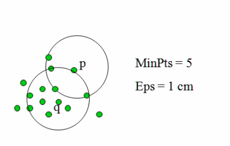
Image.1 R Clustering – R Cluster Analysis
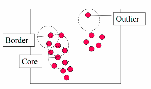
Image.2 R Clustreing – R Cluster Analysis
Once we define these parameters. The algorithm divides the data points into three points:
Core points: A point p is a core point if at least minPts points are within distance l of it (including p).
Border points: A point q is border from p if there is a path p1, …, pn with p1 = p and pn = q, where each pi+1 is reachable from pi
Outliers: All points not reachable from any other point are outliers.
The steps in DBSCAN are simple after defining the previous steps:
- First, we have to pick at random a point. That is not assigned to a cluster and then calculate its neighborhood. If, in the neighborhood, this point has minPts then make a cluster around that. Otherwise, mark it an outlier.
- As soon as we find all the core points, then we will start expanding that to include border points.
Repeat these steps until all the points are finally assigned to a cluster or to an outlier.
13. Advantages and Disadvantages of Density-based R Clustreing
Advantages:
- It does not need a predefined number of clusters.
- Basically, clusters can be of any shape, including non-spherical ones.
- Also, this technique is able to identify noise data (outliers).
- Unlike K-means, DBSCAN does not need the user to specify the number of clusters to be generated.
- DBSCAN can find any shape of clusters. Also, the cluster doesn’t have to be circular.
- DBSCAN can identify outliers.
Disadvantages
- If there are no density drops between clusters, then density-based clustering will fail.
- It seems to be difficult to detect noise points if there is variation in the density.
- It is sensitive to parameters i.e. its hard to determine the correct set of parameters.
- The quality of DBSCAN depends on the distance measure.
14. Limitation of DBSCAN
It is sensitive to the choice of e. In particular, if clusters have different densities, there are two conditions-
If e is too small then we have to define sparser clusters as noise.
e is too large- If we this condition then the denser clusters may be merged together.
c. Hierarchical R Clustering
It is an algorithm which builds a hierarchy of clusters. Although, it starts with all the data points that are assigned to a cluster of their own. Then the two nearest clusters will merge into the same cluster. In the end, we use to terminate it when there is only a single cluster left.
1. Characteristics of R Hierarchical Clustering
- Multilevel decomposition.
- The merges or splits cannot perform a rollback. Also, we can’t correct an error in an algorithm which occurs by merging.
- The hybrid algorithm.
2. Two important things that you should know about hierarchical clustering in R are:
- While we use a bottom-up approach to implement this algorithm. It is also possible to follow a top-down approach. But starting with all data points assigned to the same cluster. Hence we have to assign data point to each cluster by performing splits.
3. There are many metrics for deciding the closeness of two clusters:
Euclidean distance: ||a-b||2 = √(Σ(ai-bi))
Squared Euclidean distance: ||a-b||22 = Σ((ai-bi)2)
Manhattan distance: ||a-b||1 = Σ|ai-bi|
Maximum distance:||a-b||INFINITY = maxi|ai-bi|
Mahalanobis distance: √((a-b)T S-1 (-b)) {where, s : covariance matrix}
So, this was all in R Clustering. Hope you like our explanation.
9. Conclusion – Clustering in R
In conclusion, we have studied in detail about R Clustering and cluster analysis algorithms. Also, we saw uses, types, advantages of Clustering in R. Moreover, we have covered their applications which helps you to clarify what is a need and why to study R Clustering. Still, if you have any query regarding R Clustering, ask in the comment tab.
Did you know we work 24x7 to provide you best tutorials
Please encourage us - write a review on Google


