Clustering in R – A Survival Guide on Cluster Analysis in R for Beginners!
Job-ready Online Courses: Knowledge Awaits – Click to Access!
Previously, we had a look at graphical data analysis in R, now, it’s time to study the cluster analysis in R. We will first learn about the fundamentals of R clustering, then proceed to explore its applications, various methodologies such as similarity aggregation and also implement the Rmap package and our own K-Means clustering algorithm in R.
What is Clustering in R?
Clustering is a technique of data segmentation that partitions the data into several groups based on their similarity.
Basically, we group the data through a statistical operation. These smaller groups that are formed from the bigger data are known as clusters. These cluster exhibit the following properties:
- They are discovered while carrying out the operation and the knowledge of their number is not known in advance.
- Clusters are the aggregation of similar objects that share common characteristics.
Clustering is the most widespread and popular method of Data Analysis and Data Mining. It used in cases where the underlying input data has a colossal volume and we are tasked with finding similar subsets that can be analysed in several ways.
For example – A marketing company can categorise their customers based on their economic background, age and several other factors to sell their products, in a better way.
Get a deep insight into Descriptive Statistics in R
Applications of Clustering in R
Applications of R clustering are as follows:
- Marketing – In the area of marketing, we use clustering to explore and select customers that are potential buyers of the product. This differentiates the most likeable customers from the ones who possess the least tendency to purchase the product. After the clusters have been developed, businesses can keep a track of their customers and make necessary decisions to retain them in that cluster.
- Retail – Retail industries make use of clustering to group customers based on their preferences, style, choice of wear as well as store preferences. This allows them to manage their stores in a much more efficient manner.
- Medical Science – Medicine and health industries make use of clustering algorithms to facilitate efficient diagnosis and treatment of their patients as well as the discovery of new medicines. Based on the age, group, genetic coding of the patients, these organisations are better capable to understand diagnosis through robust clustering.
- Sociology – Clustering is used in Data Mining operations to divide people based on their demographics, lifestyle, socioeconomic status, etc. This can help the law enforcement agencies to group potential criminals and even identify them with an efficient implementation of the clustering algorithm.
In different fields, R clustering has different names, such as:
- Marketing – In marketing, ‘segmentation’ or ‘typological analyses’ term is available for clustering.
- Medicine – Clustering in medicine is known as nosology.
- Biology – It is referred to as numerical taxonomy in the field of Biology.
To define the correct criteria for clustering and making use of efficient algorithms, the general formula is as follows:
Bn(number of partitions for n objects)>exp(n)
You can determine the complexity of clustering by the number of possible combinations of objects. The complexity of the cluster depends on this number.
The basis for joining or separating objects is the distance between them. These distances are dissimilarity (when objects are far from each other) or similarity (when objects are close by).
Methods for Measuring Distance between Objects
For calculating the distance between the objects in K-means, we make use of the following types of methods:
- Euclidean Distance – It is the most widely used method for measuring the distance between the objects that are present in a multidimensional space.
In general, for an n-dimensional space, the distance is
- Squared Euclidean Distance – This is obtained by squaring the Euclidean Distance. The objects that are present at further distances are assigned greater weights.
- City-Block (Manhattan) Distance – The difference between two points in all dimensions is calculated using this method. It is similar to Euclidean Distance in many cases but it has an added functioning in the reduction of the effect in the extreme objects which do not possess squared coordinates.
The squares of the inertia are the weighted sum mean of squares of the interval of the points from the centre of the assigned cluster whose sum is calculated.
We perform the calculation of the Sum of Squares of Clusters on their centres as follows:
Total Sum of Squares (I) = Between-Cluster Sum of Squares (IR) + Within-Cluster Sum of Squares (IA)
The above formula is known as the Huygens’s Formula.
The Between-Cluster Sum of squares is calculated by evaluating the square of difference from the centre of gravity from each cluster and their addition.
We perform the calculation of the Within-Cluster Sum of squares through the process of the unearthing of the square of difference from centre of gravity for each given cluster and their addition within the single cluster. With the diminishing of the cluster, the population becomes better.
R-squared (RSQ) delineates the proportion of the sum of squares that are present in the clusters. The closer proportion is to 1, better is the clustering. However, one’s aim is not the maximisation of the costs as the result would lead to a greater number of clusters. Therefore, we require an ideal R2 that is closer to 1 but does not create many clusters. As we move from k to k+1 clusters, there is a significant increase in the value of R2
Some of the properties of efficient clustering are:
- Detecting structures that are present in the data.
- Determining optimal clusters.
- Giving out readable differentiated clusters.
- Ensuring stability of cluster even with the minor changes in data.
- Efficient processing of the large volume of data.
- Handling different data types of variables.
Note: In the case of correct clustering, either IR is large or IA is small while calculating the sum of squares.
Clustering is only restarted after we have performed data interpretation, transformation as well as the exclusion of the variables. While excluding the variable, it is simply not taken into account during the operation of clustering. This variable becomes an illustrative variable.
Wait! Have you checked – Data Types in R Programming
Agglomerative Hierarchical Clustering
In the Agglomerative Hierarchical Clustering (AHC), sequences of nested partitions of n clusters are produced. The nested partitions have an ascending order of increasing heterogeneity. We use AHC if the distance is either in an individual or a variable space. The distance between two objects or clusters must be defined while carrying out categorisation.
The algorithm for AHC is as follows:
- We first observe the initial clusters.
- In the next step, we assess the distance between the clusters.
- We then proceed to merge the most proximate clusters together and performing their replacement with a single cluster.
- We repeat step 2 until only a single cluster remains in the end.
AHC generates a type of tree called dendrogram. After splitting this dendrogram, we obtain the clusters.
Hierarchical Clustering is most widely used in identifying patterns in digital images, prediction of stock prices, text mining, etc. It is also used for researching protein sequence classification.
1. Main Distances
- Maximum distance – In this, the greatest distance between the two observed objects have clusters that are of equal diameters.
- Minimum distance – The minimum distance between the two observations delineates the neighbour technique or a single linkage AHC method.
In this case, the minimum distance between the points of different clusters is supposed to be greater than the maximum points that are present in the same cluster. The distance between the points of distance clusters is supposed to be higher than the points that are present in the same cluster.
2. Density Estimation
In density estimation, we detect the structure of the various complex clusters. The three methods for estimating density in clustering are as follows:
- The k-nearest-neighbours method – The number of k observations that are centred on x determines the density at the point x. The volume of the sphere further divides this.
- The Uniform Kernel Method – In this, the radius is fixed but the number of neighbours is not.
- The Wong Hybrid Method – We use this in the preliminary analysis.
You must definitely explore the Graphical Data Analysis with R
Clustering by Similarity Aggregation
Clustering by Similarity Aggregation is known as relational clustering which is also known by the name of Condorcet method.
With this method, we compare all the individual objects in pairs that help in building the global clustering. The principle of equivalence relation exhibits three properties – reflexivity, symmetry and transitivity.
- Reflexivity => Mii = 1
- Symmetry => Mij = Mij
- Transitivity => Mij + Mjk – Mik <=1
This type of clustering algorithm makes use of an intuitive approach. A pair of individual values (A,B) are assigned to the vectors m(A,B) and d(A,B). Both A and B possess the same value in m(A,B) whereas in the case of d(A,B), they exhibit different values.
The two individuals A and B follow the Condorcet Criterion as follows:
c(A, B) = m(A, B)-d(A, B)
For an individual A and cluster S, the Condorcet criterion is as follows:
c(A,S) = Σic(A,Bi)
The summation overall is the Bi ∈ S.
With the previous conditions, we start by constructing clusters that place each individual A in cluster S. In this cluster c(A,S), A is the largest and has the least value of 0.
In the next step, we calculate global Condorcet criterion through a summation of individuals present in A as well as the cluster SA which contains them.
Note: Several iterations follow until we reach the specified largest number of iterations or the global Condorcet criterion no more improves.
K-Means Clustering in R
One of the most popular partitioning algorithms in clustering is the K-means cluster analysis in R. It is an unsupervised learning algorithm. It tries to cluster data based on their similarity. Also, we have specified the number of clusters and we want that the data must be grouped into the same clusters. The algorithm assigns each observation to a cluster and also finds the centroid of each cluster.
The K-means Algorithm:
- Selects K centroids (K rows chosen at random).
- Then, we have to assign each data point to its closest centroid.
- Moreover, it recalculates the centroids as the average of all data points in a cluster.
- Assigns data points to their closest centroids.
- Moreover, we have to continue steps 3 and 4 until the observations are not reassigned.

This algorithm works in these steps:
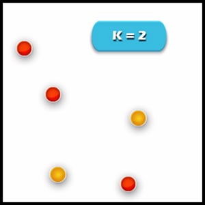
1. Specify the desired number of clusters K: Let us choose k=2 for these 5 data points in 2D space.
2. Assign each data point to a cluster: Let’s assign three points in cluster 1 using red colour and two points in cluster 2 using yellow colour (as shown in the image).
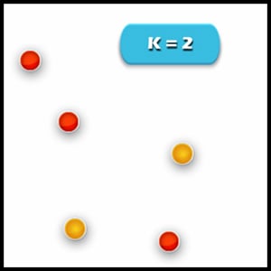
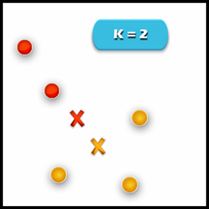
3. Compute cluster centroids: The centroid of data points in the red cluster is shown using the red cross and those in a yellow cluster using a yellow cross.
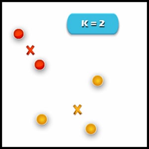
4. Re-assignment of points to their closest cluster in centroid: Red clusters contain data points that are assigned to the bottom even though it’s closer to the centroid of the yellow cluster. Thus, we assign that data point into a yellow cluster.
5. Re-compute cluster centroids: Now, re-computing the centroids for both the clusters. We perform the repetition of step 4 and 5 and until that time no more improvements can be performed. We’ll repeat the 4th and 5th steps until we’ll reach global optima. This continues until no more switching is possible. Then it will mark the termination of the algorithm if not mentioned.
We will now understand the k-means algorithm with the following example:
> #Author DataFlair
> library(tidyverse)
> library(cluster)
> library(factoextra)
> library(gridExtra)
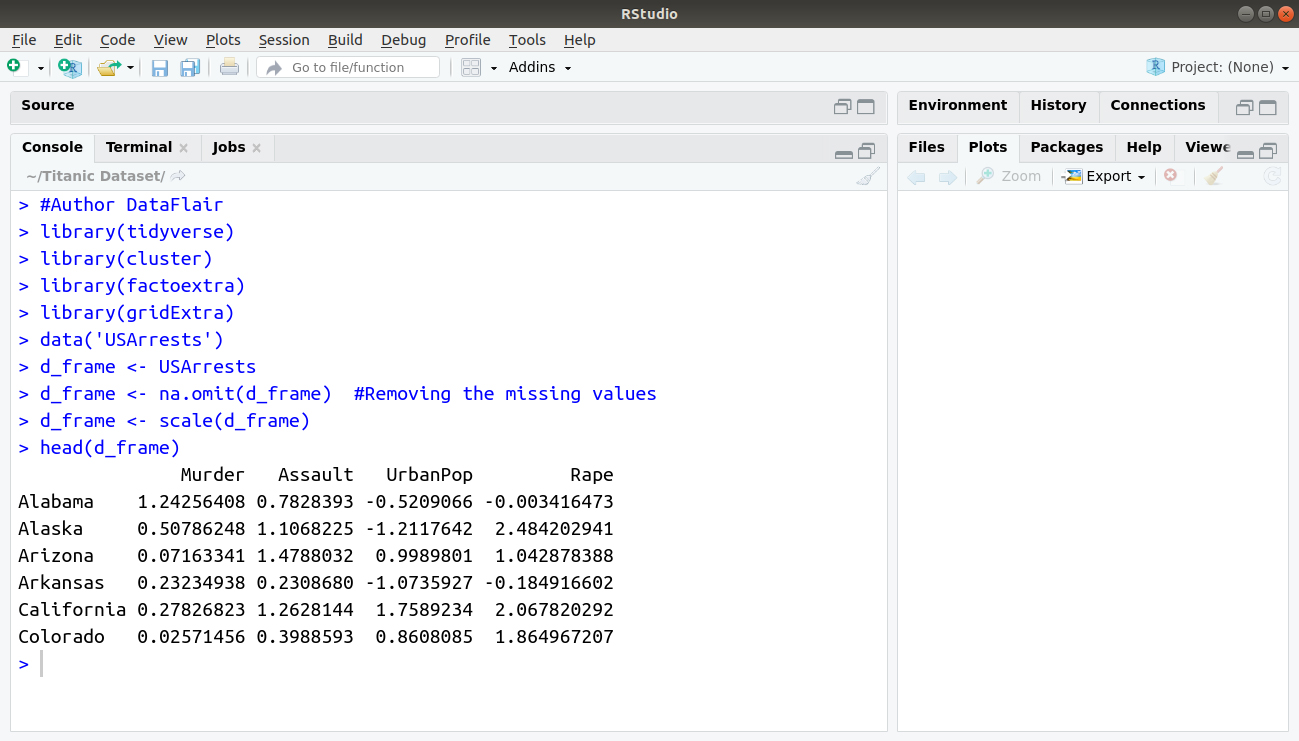
> data('USArrests')
> d_frame <- USArrests
> d_frame <- na.omit(d_frame) #Removing the missing values
> d_frame <- scale(d_frame)
> head(d_frame)
Output:
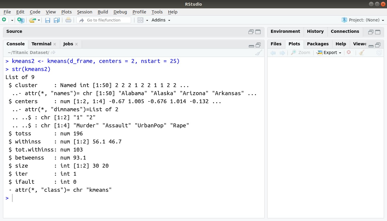
> kmeans2 <- kmeans(d_frame, centers = 2, nstart = 25)
> str(kmeans2)
Output:
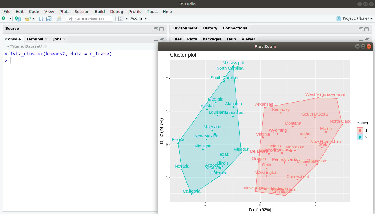
> fviz_cluster(kmeans2, data = d_frame)
Output:
> kmeans3 <- kmeans(d_frame, centers = 3, nstart = 25)  #DataFlair
> kmeans4 <- kmeans(d_frame, centers = 4, nstart = 25)
> kmeans5 <- kmeans(d_frame, centers = 5, nstart = 25)
> #Comparing the Plots
> plot1 <- fviz_cluster(kmeans2, geom = "point", data = d_frame) + ggtitle("k = 2")
> plot2 <- fviz_cluster(kmeans3, geom = "point", data = d_frame) + ggtitle("k = 3")
> plot3 <- fviz_cluster(kmeans4, geom = "point", data = d_frame) + ggtitle("k = 4")
> plot4 <- fviz_cluster(kmeans5, geom = "point", data = d_frame) + ggtitle("k = 5")
> grid.arrange(plot1, plot2, plot3, plot4, nrow = 2)
Output:

Cyber Profiling with K-Means Clustering
Conventionally, in order to hire employees, companies would perform a manual background check. This type of check was time-consuming and could no take many factors into consideration. However, with the help of machine learning algorithms, it is now possible to automate this task and select employees whose background and views are homogeneous with the company. In cases like these cluster analysis methods like the k-means can be used to segregate candidates based on their key characteristics.
With the new approach towards cyber profiling, it is possible to classify the web-content using the preferences of the data user. This preference is taken into consideration as an initial grouping of the input data such that the resulting cluster will provide the profile of the users. The data is retrieved from the log of web-pages that were accessed by the user during their stay at the institution.
Summary
In the R clustering tutorial, we went through the various concepts of clustering in R. We also studied a case example where clustering can be used to hire employees at an organisation. We went through a short tutorial on K-means clustering.
The upcoming tutorial for our R DataFlair Tutorial Series – Classification in R
If you have any question related to this article, feel free to share with us in the comment section below.
If you are Happy with DataFlair, do not forget to make us happy with your positive feedback on Google


Hi there… I tried to copy and paste the code but I got an error on this line
grpMeat <- kmeans(food[,c("WhiteMeat","RedMeat")], centers=3, + nstart=10)
the error specified:
Error: unexpected '=' in "grpMeat <- kmeans(food[,c("WhiteMeat","RedMeat")], centers=3, + nstart="
if you have the csv file can it be available in your tutorial? Thanks a lot
http://www.biz.uiowa.edu/faculty/jledolter/DataMining/protein.csv
thank you so much bro for this blog it’s really helpfull
i have two questions about k-means clustring
1 – Can I predict groups of new individuals after clustering using k-means algorithm ?
2 – assuming I have the clusters of the k-means method, can we create a table represents the individuals from each one of the clusters
Really helpful in understanding and implementing.
which kind of clustering method, do you recommend if i have non-normal data and i need work with outliers?
Thanks a million.
I needed this to understand clustering. I surely have to practice this.
Wow…
This is super-helpful.
I really needed this to understand clustering.
Thanks a million.
Very helpful..
Thanks alot.