Data Manipulation in R – Find all its concepts at a single place!
Placement-ready Online Courses: Your Passport to Excellence - Start Now
We will learn how to perform data manipulation in R programming language along with data processing. We will also overview the three operators such as subsetting, manipulation as well as sorting and merging in R. Also, we will learn about data structures in R, how to create subsets in R and usage of R sample() command, ways to create R data subgroups or bins of data in R. We will also overview the different methodologies for aggregating data in R, performing sorting, ordering as well as data traversal.
These R data manipulation topics will provide you with a complete tutorial on ways for manipulating and processing data in R.
What is Data Manipulation in R?
With the help of data structures, we can represent data in the form of data analytics. Data Manipulation in R can be carried out for further analysis and visualisation.
Before we start playing with data in R, you must learn how to import data in R and ways to export data from R to different external sources like SAS, SPSS, text file or CSV file.
One of the most important aspects of computing with Data Manipulation in R is that it enables its subsequent analysis and visualization. Let us see a few basic data structures in R:
1. Vectors in R
These are ordered containers of primitive elements and are used for 1-dimensional data.
Types – integer, numeric, logical, character, complex.
2. Matrices in R
These are rectangular collections of elements and are useful when all data is of a single class that is numeric or characters.
Dimensions – two, three, etc.
3. Lists in R
These are ordered containers for arbitrary elements and are used for higher dimension data, like customer data information of an organization. When data cannot be represented as an array or a data frame, the list is the best choice. This is because lists can contain all kinds of other objects, including other lists or data frames, and in that sense, they are very flexible.
Learn what all you can do with Lists in R Programming
4. Data Frames
These are two-dimensional containers for records and variables and are used for representing data from spreadsheets etc. It is similar to a single table in the database.
Creating Subsets of Data in R
As we know, data size is increasing exponentially and doing an analysis of complete data is very time-consuming. So, the data is divided into small-sized samples and analysis of samples is done. The process of creating samples is called subsetting.
Different methods of subsetting in R are:
1. $
The dollar sign operator selects a single element of data. The result of this operator is always a vector when we use it with a data-frame.
2. [[
Similar to $ in R, the double square brackets operator in R also returns a single element, but it offers the flexibility of referring to the elements by position rather than by name. It can be used for data frames and lists.
3. [
The single square bracket operator in R returns multiple elements of data. The index within the square brackets can be a numeric vector, a logical vector, or a character vector.
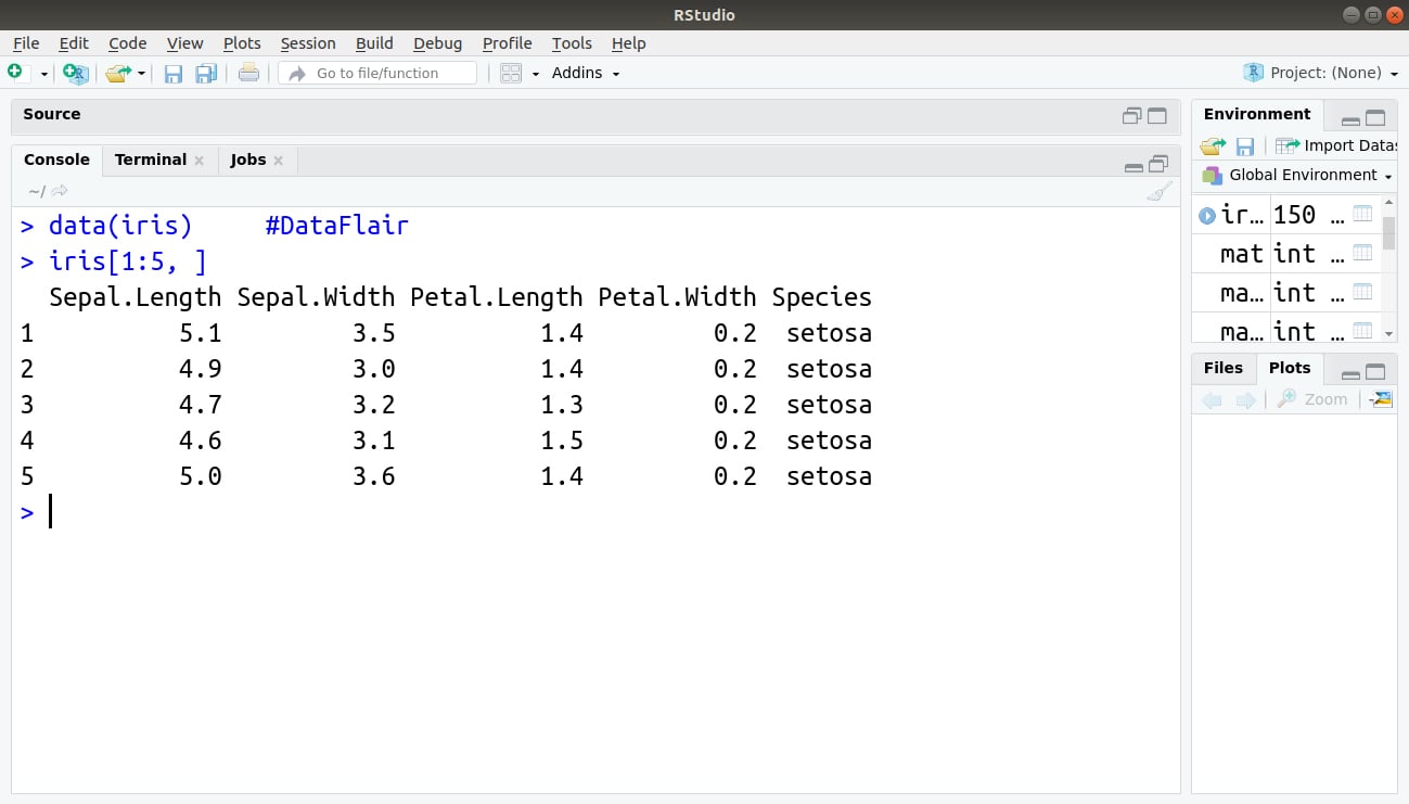
For example: To retrieve 5 rows and all columns of already built-in dataset iris, the below command, is used:
> data(iris)
> iris[1:5, ]
Output:
sample() command in R
As we have seen, samples are created from data for analysis. To create samples, sample() command is used and the number of samples to be drawn are mentioned.
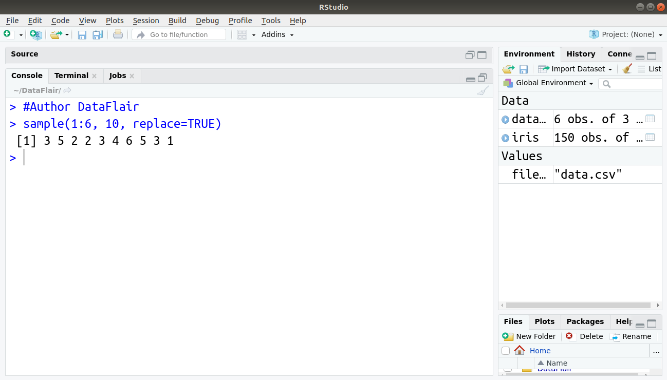
For example, to create a sample of 10 simulations of a die, below command is used:
> sample(1:6, 10, replace=TRUE)
Output:
sample() should always produce random values but it does not happen with the test code sometimes. If substituted with a seed value, the sample() command always produces random samples.
The seed value is the starting point for any random number generator formula. Seed value defines both, the initialization of the random number generator along with the path that the formula will follow.
Let us see how seed value is used:
> set.seed(100)
> sample(1:5, 10, replace = TRUE) #DataFlair
Gain Expertise in the Numeric and Character Functions in R
Applications of Subsetting Data
Let us now see a few applications of subsetting data in R:
1. Duplicate data can be removed during analysis using duplicated()function in R
Below command shows how to find duplicate data in subsets: duplicated() function finds duplicate values and returns a logical vector that tells you whether the specified value is a duplicate of a previous value.
> duplicated(c(1,2,1,3,1,4))
Output:
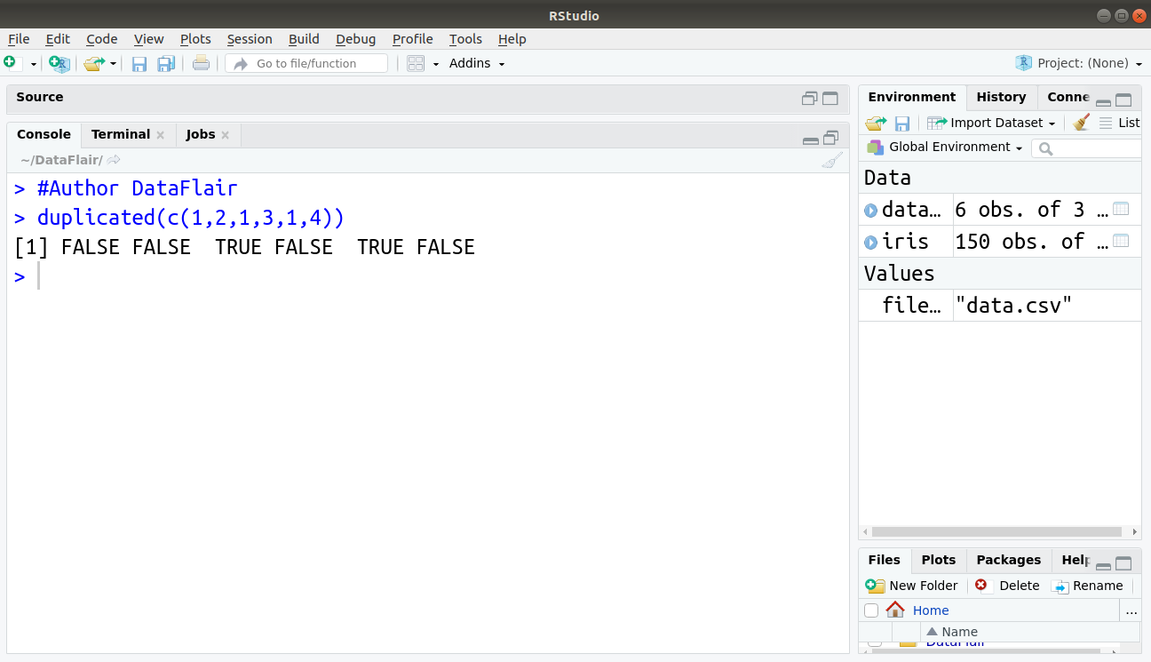
For all those values which are duplicate in the sample, true is returned.
2. Missing data can be identified using complete.cases() function in R
During analysis, any row with missing data can be identified and removed as below.
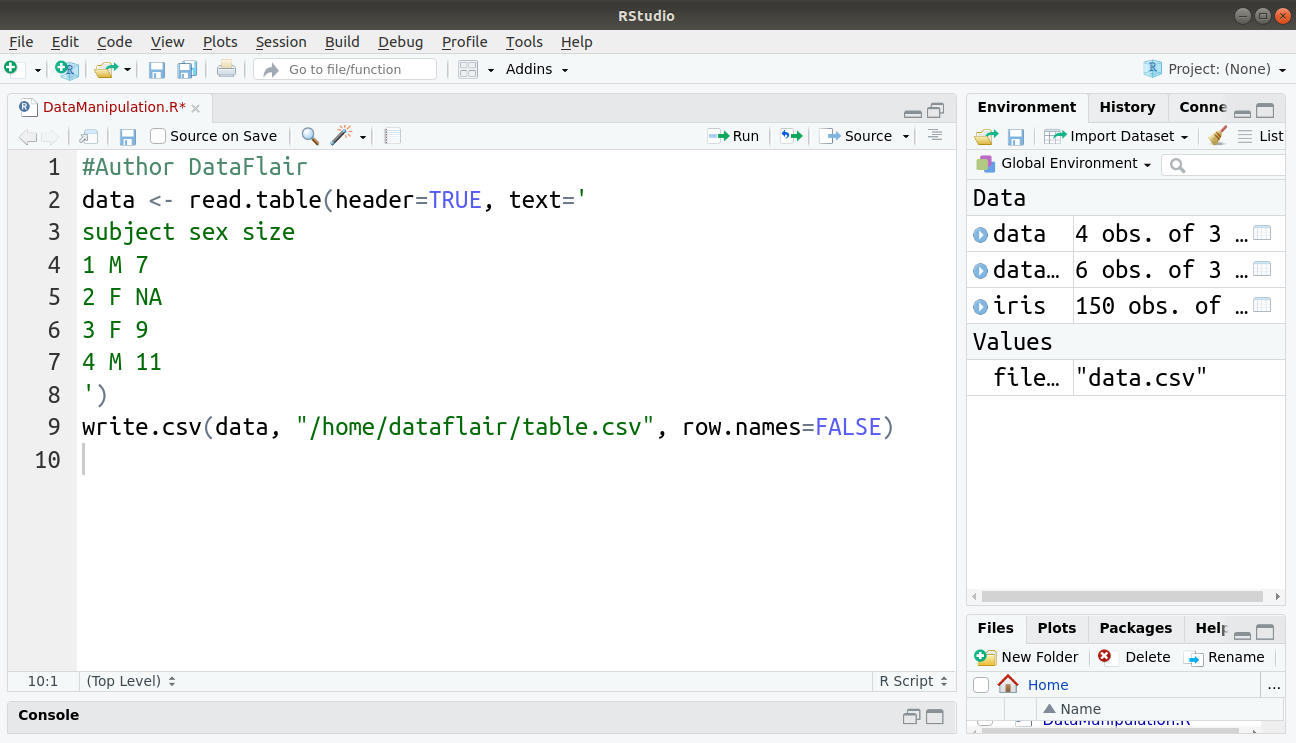
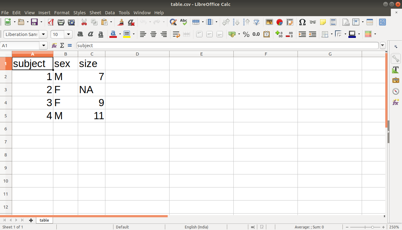
complete.cases() command in R is used to find rows which are complete. It gives logical vector with the value TRUE for rows that are complete, and FALSE for rows that have some NA values. We will first create our data and store it in a CSV file as follows:
#Author DataFlair
data <- read.table(header=TRUE, text='
subject sex size
1 M 7
2 F NA
3 F 9
4 M 11
')
write.csv(data, "/home/dataflair/table.csv", row.names=FALSE)
Code Display:
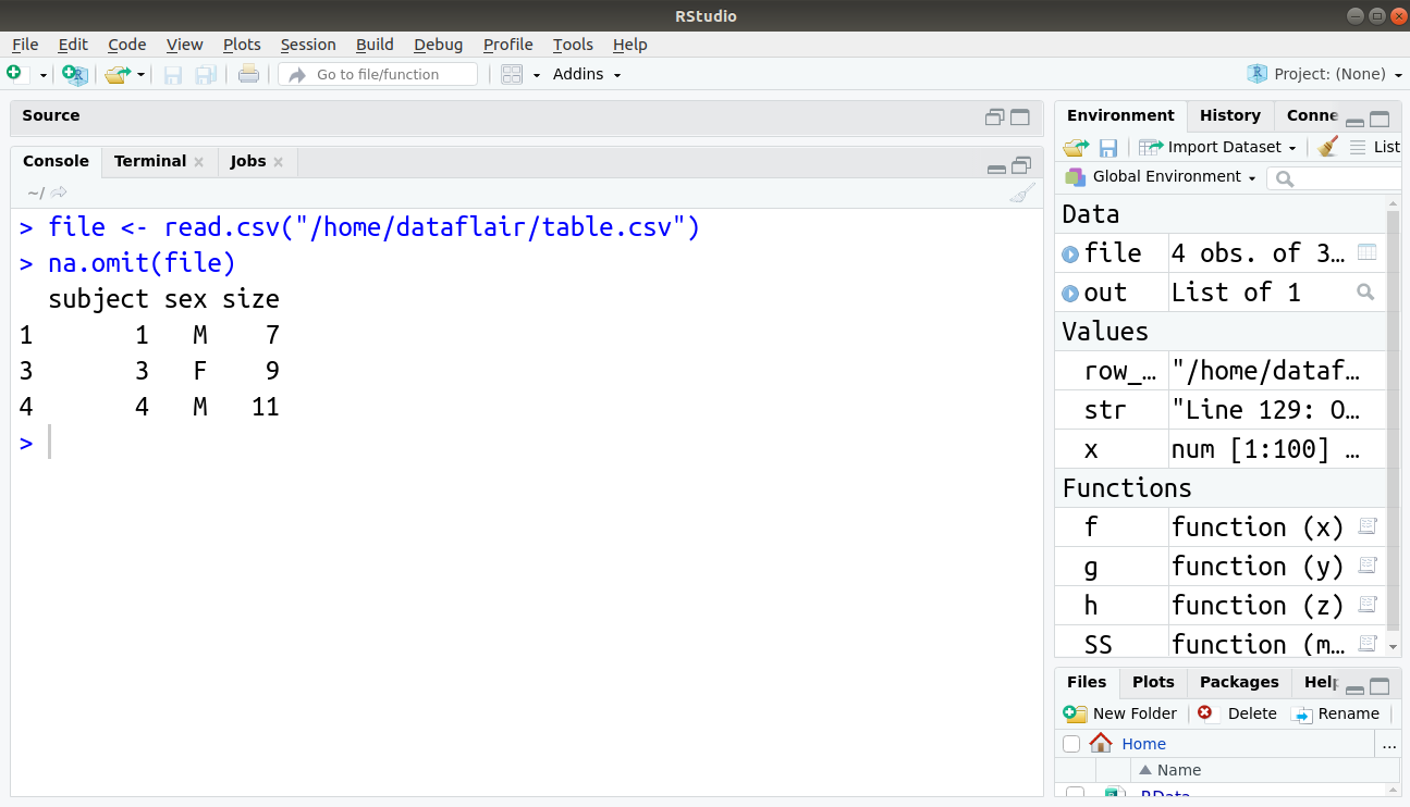
Rows which have NA values can be removed using the na.omit() function as below:
> file <- read.csv("/home/dataflair/table.csv")
> na.omit(file)
Output:
Adding Calculated Fields to Data
After creating the appropriate subset of your data, the next step in your analysis is to perform some calculations. R makes it easy to perform calculations on columns of a data frame because each column is itself a vector.
Let us see data manipulation with R with the help of an example:
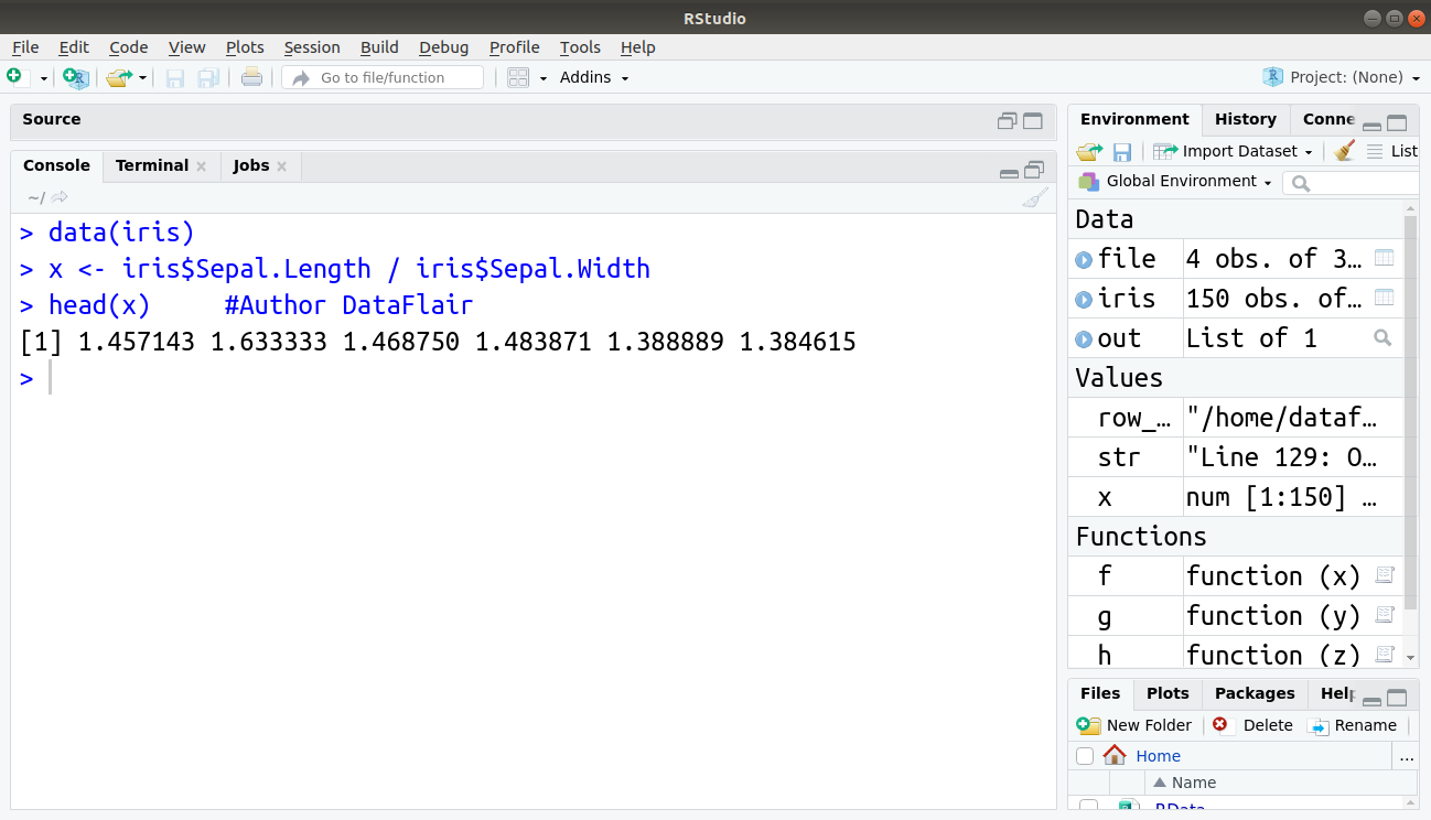
We will see how to calculate the ratio between the lengths and width of the sepals.
The command for the same is:
> data(iris)
> x <- iris$Sepal.Length / iris$Sepal.Width
> head(x)     #Author DataFlair
Output:
1. with() function in R
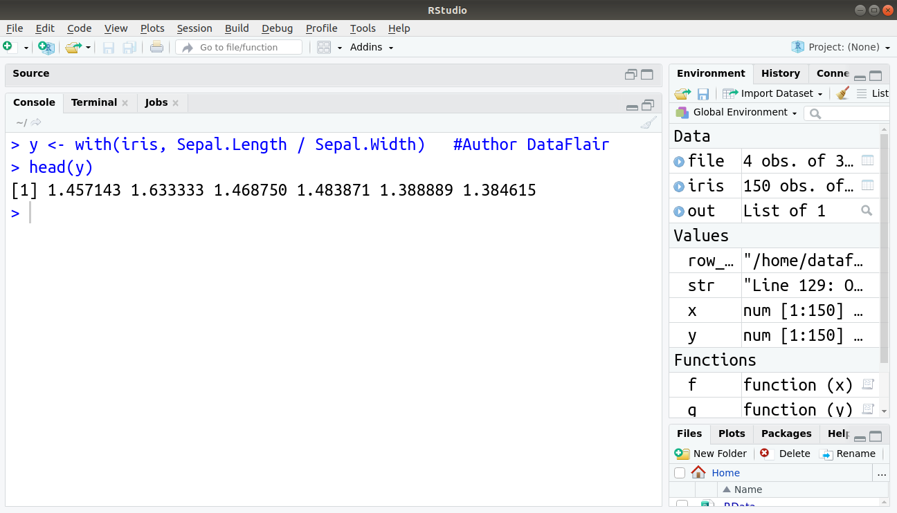
To reduce the amount of typing and make the code more readable, we use with() command as below:
> y <- with(iris, Sepal.Length / Sepal.Width)   #Author DataFlair
> head(y)
This gives output same as above but reduces the task of typing.
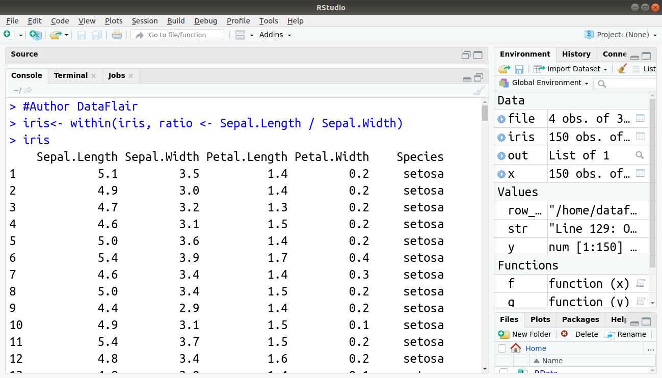
2. within() function in R
Let us now see the use of within() function for the same task:
iris<- within(iris, ratio <- Sepal.Length / Sepal.Width)
iris
Output:
with() function allows you to refer to columns inside a data frame without explicitly using the dollar sign or even the name of the data frame itself.
We can use with() and within() interchangeably.
You must have a look at R Vector Functions
Creating Subgroups or Bins of Data
Most statisticians often draw histograms to investigate their data. As this type of calculation is common when you use statistics, R has some functions for it.
1. cut() function in R
cut() function groups values of a variable into larger bins. It creates bins of equal size and classifies each element into its appropriate bin.
Let us see how cut works in R with an example:
> #Author DataFlair
> frost <- c(1,2,3)
> cut(frost, 3, include.lowest=TRUE)
> cut(frost, 3, include.lowest=TRUE, labels=c("Low", "Med", "High"))
Output:

This gives the result as a factor with three levels. The cut() function creates mathematical labels for the bins. The label names can be provided by the user.
The result shows three labels in the output.
2. table() function in R
To count the number of observations in each level of factor, we can use the R table() command as below:
> inp <- cut(frost, 3, include.lowest=TRUE, labels=c("Low", "Med", "High"))     #Author DataFlair
> table(inp)
Output:
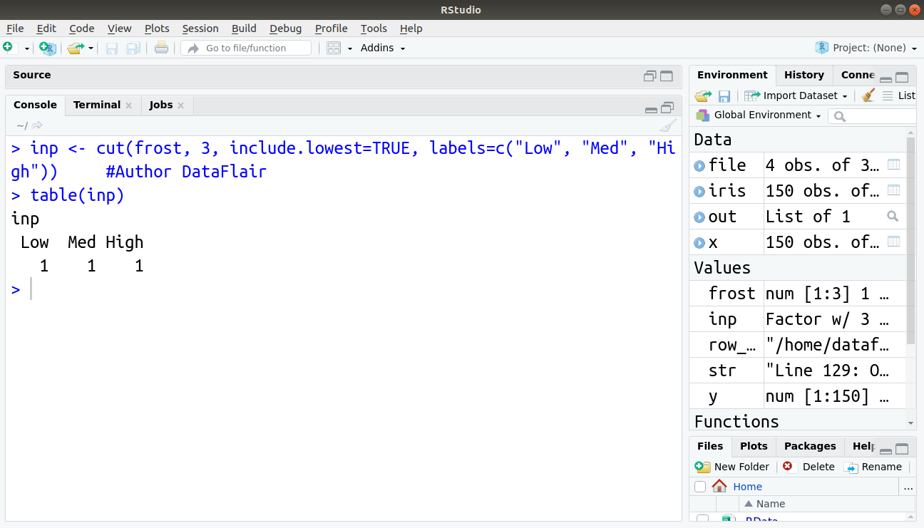
The result shows the output as a table containing the number of elements in each factor. Now let see combining and merging datasets for data manipulation in R.
Combining and Merging Datasets in R
If you want to combine data from different sources in R, you can combine different sets of data in three ways:
1. By Adding Columns using cbind() in R
If the two sets of data have an equal set of rows, and the order of the rows is identical, then adding columns makes sense. This can be done by using the data.frame or cbind() function.
2. By Adding Rows using rbind() function in R
If both sets of data have the same columns and you want to add rows to the bottom, then use rbind().
3. By Combining Data With Different Shapes using merge() function in R
The merge() function combines data based on common columns as well as rows. In database language, this is usually called joining data.
For merging the existing data, using merge() function is useful. You can use merge() to combine data only when certain matching conditions are satisfied.
merge() Function in R
Let’s see the use of merge() function.
The merge() function is used to combine data frames. Let us see this with an example:
#Author DataFlair
every.states <- as.data.frame(state.x77)
every.states$Name <- rownames(state.x77)
rownames(every.states) <- NULL
str(every.states)
#Creating a subset of freezing states
freezing.states <- every.states[every.states$Frost>150
                                , c("Name", "Frost")]
freezing.states
#Creating a subset of big states
big.states <- every.states[every.states$Area>=100000
                           , c("Name", "Area")]
big.states
#Using the merge function
merge(freezing.states, big.states)
Output:

This is the command to create a data frame that consists of cold as well as large states.
Let us see different types of merge().
The merge() function allows four ways of combining data:
1. Natural Join in R
To keep only that rows which match from the data frames, specify the argument all=FALSE.
2. Full Outer Join in R
To keep all the rows from both the data frames, specify all=TRUE.
3. Left Outer Join in R
To include all the rows of your data frame x and only those from y that match, specify all.x=TRUE.
4. Right Outer Join in R
To include all the rows of your data frame y and only those from x that match, specify all.y=TRUE
The merge()function takes a large number of arguments, as follows:
- x: A data frame.
- y: A data frame.
- by, by.x, by.y: Names of the columns are common to both x and y. By default, it uses columns with common names between the two data frames.
- all, all.x, all.y: Logical values that specify the type of merge. The default value is all = FALSE.
Any doubts in R Data Manipulation till now? Please comment below.
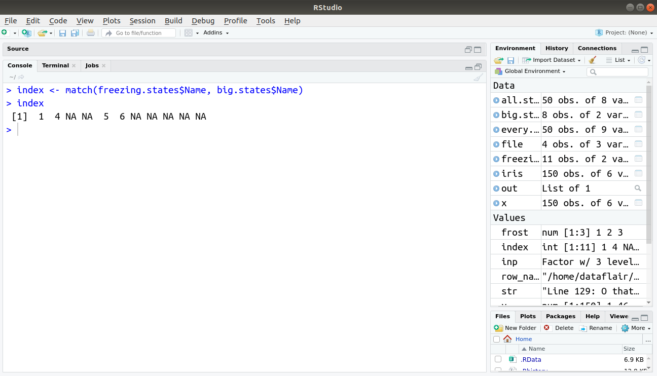
match() function in R
The R match() function returns the matching positions of two vectors or, more specifically, the positions of the first matches of one vector in the second vector.
> index <- match(freezing.states$Name, big.states$Name)
> index
Output:
Sorting and Ordering Data in R using sort() and order() in R
A common task in data analysis and reporting is sorting information. You can answer many everyday questions with sorted tables of data that tell you the best or worst of specific things; for example, parents want to know which school in their area is the best, and businesses need to know the most productive factories of the most lucrative sales areas.
Let’s first create data frame and then we will sort it. Then, we will use some.states command to create a data frame.
#Author DataFlair
some.states <- data.frame( Region = state.region, + state.x77)
some.states <- some.states[1:10, 1:3]
sort(some.states$Population)   #Command to sort Population in ascending order
sort(some.states$Population, decreasing=TRUE)   #Command to sort Population
                                                #in descending order
order.pop <- order(some.states$Population)      #Another way of sorting
some.states[order.pop, ]        #In ascending order
order(some.states$Population, decreasing=TRUE)   #Descending Order
Output:
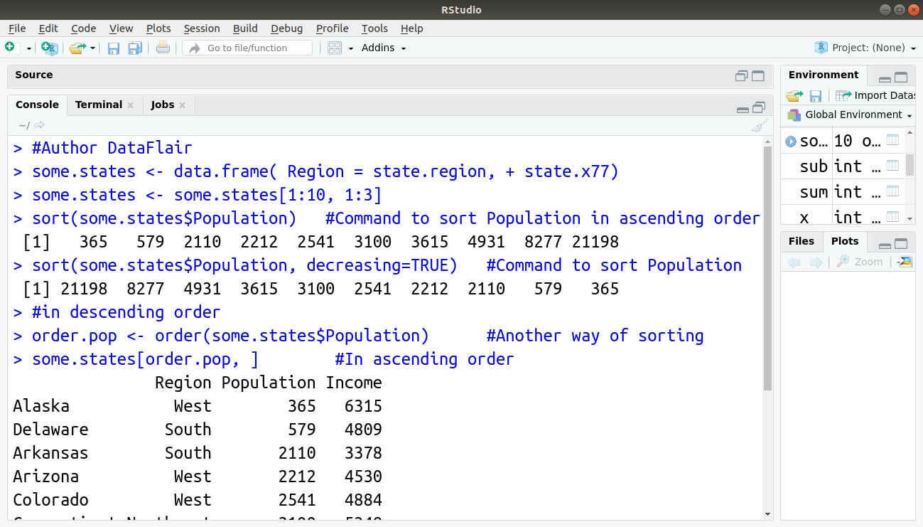
This is how we use the order() and sort() functions.
Get a deep insight into the Characteristics of R Data Frame
Traversing Data with the Apply() Function in R
To traverse the data, R uses the apply functions. The output of the apply() function depends on the data structure being traversed.
1. Array or Matrix
The apply() function traverses either the rows or columns of a matrix, applies a function to each resulting vector, and returns a vector of summarized results
2. List
The lapply() function can traverse a list. It applies a function to each element and returns a list of the results. Sometimes, it is possible to simplify the resulting list into a matrix or vector. lapply returns a list of the same length as X, each element of which is the result of applying FUN to the corresponding element of X.
Use the R apply() function as below:
apply(X, MARGIN, FUN, ...)
The apply() function takes four arguments as below:
- X: This is the data-an array (or matrix).
- MARGIN: This is a numeric vector that indicates the dimension over which to traverse-1 means rows and 2 means columns.
- FUN: This is the function to apply (for example, sum or mean).
- … (dots): If the FUN function requires any additional arguments, they can be added here.
In essence, the apply function allows us to make entry-by-entry changes to data frames and matrices. If MARGIN=1, the function accepts each row of X as a vector argument and returns a vector of the results. Similarly, if MARGIN=2, the function acts on the columns of X most appropriately, when we apply MARGIN=c(1,2) function to every entry of X.
Let us now discuss the variations of the apply() function:
1. lapply() function in R
We have already seen it above.
2. sapply() function in R
It works on a list or vector and returns vector.
3. tapply() function in R
We use it to create tabular summaries of data. This function takes three arguments:
- X: Refers to a vector.
- INDEX: Refers to a factor or list of factors.
- FUN: Refers to a function.
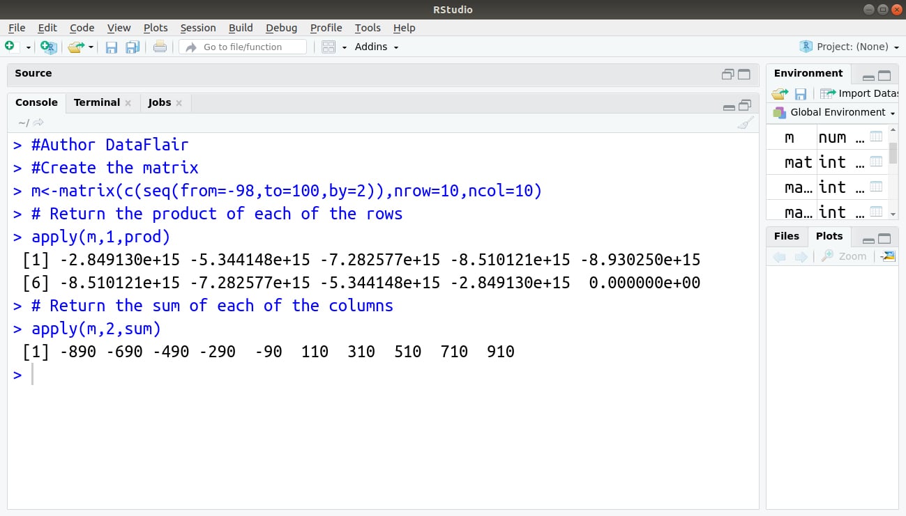
An illustrative example:
#Author DataFlair
#Create the matrix
m<-matrix(c(seq(from=-98,to=100,by=2)),nrow=10,ncol=10)
# Return the product of each of the rows
apply(m,1,prod)
# Return the sum of each of the columns
apply(m,2,sum)
Output:
Don’t forget to check the Factor Analysis in R Programming
Formula Interface in R
The R formula interface allows you to concisely specify which columns to use when fitting a model, as well as the behaviour of the model for data manipulation in R.
You need the operators when you start building models. Formula notation refers to statistical formulae, as opposed to mathematical formulae. The formula operator ‘+’ means to include a column, not to mathematically add two columns together.
| Operator | Example | Meaning |
| ~ | y ~ x | Model y as a function of x. |
| + | y ~ a + b | Include columns a as well as b. |
| – | y ~ a – b | Include a but exclude b. |
| : | y ~ a : b | Estimate the interaction of a and b. |
| * | y ~ a * b | Include columns as well as their interaction (that is, y ~ a + b + a:b). |
| | | y ~ a | b | Estimate y as a function of a conditional on b. |
Above table shows the meaning of different operators in formula interfacing.
Variables in R
The two types of R variables are:
1. Identifier Variables in R
Identifier or ID variables identify the observations. These act as the keys that identify the observations.
2. Measured Variables in R
These represent the measurements to observe.
Reshape2 Package in R
Base R has a function, reshape() that works fine for reshaping longitudinal data.
The problem of data reshaping is far more generic than simply dealing with longitudinal data. So, package reshape2 that contains several functions to convert data between long and wide format is released.
> install.packages("reshape2")
> library(reshape2)
R reshape2 package is based on two key functions:
- Melt() in R takes wide-format data and melts it into long-format data.
- Cast() in R takes long-format data and casts it into wide-format data.
Summary
In this tutorial on data manipulation in R, we discussed the methods of creating subsets of data in R. Moreover, we saw sample() command in R, applications of subsetting data, creating subgroups or bins of data, combining and merging datasets in R and much more.
Now, it’s time for exploring the Descriptive Statistics in R for Data Frames
Was the article useful for you? Do share your thoughts in the comment section below. We will be glad to hear from you🙂
Your 15 seconds will encourage us to work even harder
Please share your happy experience on Google


This is really a nice tutorial. I have never used with or within, I will give it a go. Thanks