R Graphical Models Tutorial for Beginners – A Must Learn Concept!
Job-ready Online Courses: Click, Learn, Succeed, Start Now!
This tutorial will provide you with a detailed explanation of graphical models in R programming. First of all, we will discuss about the graphical model concept, its types and real-life applications then, we will study about conditional independence and separation in graphs, and decomposition with directed and undirected graphs.
So, let’s start.
What is R Graphical Models?
R graphical models refer to a graph that represents relationships among a set of variables. By a set of nodes (vertices) and edges, we design these models to connect those nodes.
Define a graph G by the following equation:
G = (V, E)
Here:
- V is a finite set of vertices or nodes.
- E ⊆ V × V is a finite set of edges, links, or arcs.
A graphical model encodes conditional independence assumptions between variables. It represents random variables as nodes or vertices and conditional independence assumptions as missing arcs.
First, confirm that you have completed – Contingency Tables in R Programming
Some real-life examples of graphical models using nodes and edges are:
- Road Maps – Represent crossings and streets.
- Electrical Circuits – Represent electronic components and edges.
- Computer Networks – Represent computers and connections.
- World Wide Web – Represent web pages and links.
- Flowcharts – Represent boxes and arrows.
R graphical models represent a class of probability distribution in terms of a graph. They combine uncertainty and logical structure into a credible, real-world phenomenon. They provide an effective way to connect the dots and reason the unlimited observations and variable available around us.
It is a probabilistic model for which a graph denotes the dependence structure between random variables. They are commonly used in probability theory, statistics particularly Bayesian statistics and Machine Learning to specify the dependencies in a domain under study. The conditional distribution functions that represent the quantitative information about the domain at the end estimate its need. This approach is tiresome and time-consuming. For example – Large domains like retail which have 1000 variables.
Let us see in the given image x ∈ X, how the human pose estimates in image y ∈ Y.
The computation starts with the estimation of different body parts, as follows.
The formula to calculate the body part, for example estimating head, yhead = (u; v; Θ) where:
- (u; v) center, where: (u; v) ∈ {1,….,M} X {1,….,N};
- Θ rotation, where: Θ ∈ {0, 45˚, 90˚,…};
As shown in the figure, estimate a head classifier as:
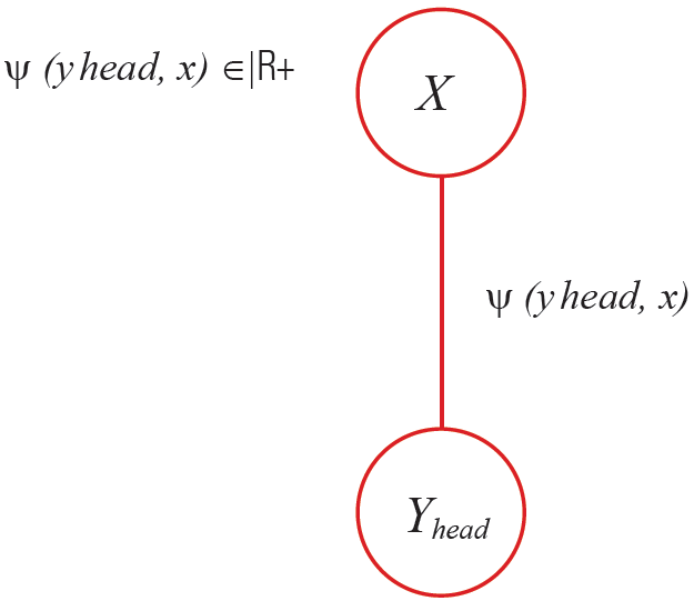
- With this classifier, check a score and record for all positions in the picture.
- Repeat this process for all the body parts and repeat until the entire image for different body classifiers scans, as shown in the figure in the following slide:
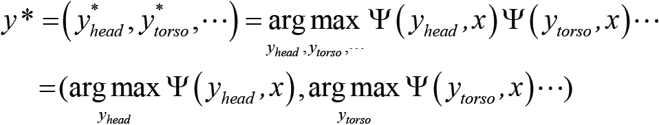
Predict the most precise human pose as:
- To capture the uncertainty of a phenomenon given by some data, we use probability distribution as:

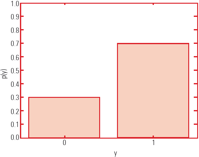
- The following slide shows an example of the probability distribution graph.
- The graph depicts a binary variable, which is y ∈ Y = {0.1}.
- It has 2 values and 1 degree of freedom.
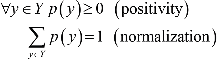
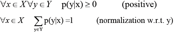
In this graph, the conditional probability distribution is:
Learn to Implement Functions of Normal Distribution in R
Types of R Graphical Models
There are two main types of graphical models in R:
- Undirected Graphical Models [Markow Random Fields (MRFs)] – In this case of Markov Networks, they are based on an undirected graph. Due to this, they are known as undirected graphical models.
- Directed or Bayesian Networks – In this case, the Bayesian Networks are based on the directed graphs. Therefore, they are referred to as directed R graphical models.
Both families encompass the properties of factorization and independences. They differ in the set of independences they can encode and the factorization of the distribution that they induce.
1. Undirected R Graphical Models
An undirected graph is the one whose edges do not possess any form of orientation. In this graph, the edge of (a,b) is identical to edge(b,a). This means that they are not ordered but have two sets of vertices. The largest number of edges in an undirected graph without a self-loop is n(n – 1)/2.
A graph G is indirect if ∀A, B ∈ V: (A, B) ∈ E ⇒ (B, A) ∈ E.
Identify the two ordered pairs (A, B) and (B, A) and represent by only one undirected edge.
A type of model that is over an undirected graph is a Markov Network, otherwise known as Markov Random Field.
These models can be used for modeling a variety of phenomena where one cannot ascribe a directionality to the interaction between variables. With the help of undirected graphs, we can have a much simpler perspective on the directed model. They share the terms of independence structure as well as the inference task.
MRF is an undirected conditional independence graph of a probability distribution. The probability distribution along the family of non-negative functions M consists of the factorisation created by the graph.
Suppose that G = (V, E).
Here, vertex set V = {0,1,2,3,4,5,6} and edge set E = {(0,2), (0,4), (0,5), (1,0), (2,1), (2,5), (3,1), (3,6), (4,0), (4,5),(6,3),(6,5)}.
1.1 Undirected Graph Terminology
Let us see few terminologies related to undirected graph:
1. Adjacent Node – A node B ∈ V is adjacent to a node A ∈ V or a neighbor of A.
If and only if there is an edge between them, then (A, B) ∈ E.
Two nodes are adjacent if they share a common edge in which case the common edge is to join the two vertices. The two endpoints of an edge are also said to be next to each other.
2. Set of neighbors – The set of all neighbors of A is neighbors (A) = {B ∈ V | (A,B) ∈ E}. The set neighbors(A) is sometimes also called the boundary of A.
3. Degree of node – The degree of the node A (number of incident edges) is deg(A) = | neighbors(A)|. The degree of a node is the number of edges that connect to it, where an edge that connects to the node at both ends (a loop). Count the edge twice. The degree of a vertex is a measure of immediate adjacency.
4. Closure of node – The closure of node A is the boundary of A together with A itself. closure(A) = neighbors(A) ∪ {A}.
5. Connected nodes – Two distinct nodes A, B ∈ V are called connected in G if and only if there exists a sequence C1, . ., Ck, k ≥ 2, of distinct nodes, called a path, with C1 = A, Ck = B, and ∀i, 1 ≤ i < k : (Ci, Ci+1) ∈ E.
6. Tree – An undirected graph is singly connected or a tree if and connect only if any pair of distinct nodes is by exactly one path. The tree serves the role of a connected graph that contains no cycles. Connect end 2 vertices by exactly 1 simple path.
7. Subgraph – A subgraph is a subset of a graph’s edges (and associated vertices) that forms a graph. An undirected graph GX = (X, EX) is called a subgraph of G (induced by X)if and only if X ⊆ V and EX = (X×X) ∩ E, that is if it contains a subset of the nodes in G and all corresponding edges.
8. Complete graph – The complete graph Kn of order n is a simple graph with n vertices in which every vertex is next to every other. An undirected graph G = (V, E) is complete if its set of edges is complete, that is, if all possible edges are present, or if: E = V × V − {(A, A) | A ∈ V}.
9. Clique – A clique in a graph is a set of pairwise adjacent vertices. The two subgraphs of clique and a complete subgraph are used interchangeably as a subgraph itself by a clique is a complete subgraph. A complete subgraph is called a clique. A clique is maximal if it is not a subgraph of a larger clique, that is, a clique having more nodes.
You must explore the Graphical Models Applications
2. Directed R Graphical Models
A directed graph or digraph is an ordered pair D = (V,A) with:
- V set whose elements are called vertices or nodes, and
- A set of ordered pairs of vertices, called arcs, directed edges, or arrows.
Let us assume an edge (A,B) and direct it towards B from A.
Directed R graphical models are also called Bayesian networks or Bayes nets (BN).
A Bayesian network is a directed conditional independence graph of a probability distribution. It is along with the family of conditional probabilities of the factorization brought by the graph.
A Bayesian network, Bayes network, belief network, Bayes(ian) model is a probabilistic graphical model. It represents a set of random variables and their conditional dependencies via a directed acyclic graph (DAG). For example – It could represent the probabilistic relationships between diseases and symptoms. Given symptoms, the network can be used to compute the probabilities of the presence of various diseases.
Suppose, vertex set V = {0,1,2,3,4,5,6} and edge set E = {(0,2), (0,4), (0,5), (1,0), (2,1), (2,5), (3,1), (3,6), (4,0), (4,5), (6,3), (6,5)}. We can create a directed graph from it.
Time to master the concept of Bayesian Network in R
2.1 Directed Graph Terminologies
Let us see a few terms related to the directed graph:
- Parent and child note – Given an edge, the node that the edge points from is called the parent and the node that the edge points to is called the child. A node B ∈ V is called a parent of a node A ∈ V. A is called the child of B, if there is a directed edge from B to A, that is, if and only if (B, A) ∈ E.
B is called adjacent to A, if it is either a parent or a child of A and denotes the set of all parents of a node A:
parents(A) = {B ∈ V | (B,A) ∈ E}
Denote the set of its children:
children(A) = {B ∈ V | (A,B) ∈ E}
- D-connected nodes – Two nodes A, B ∈ V are called d-connected in G, if there is a sequence C1, ., Ck, k ≥ 2, of distinct nodes, called a directed path, with C1 = A, Ck = B, and ∀i, 1 ≤ i< k : (Ci, Ci+1) ∈ E .
x and y are d-connected if there is an unblocked path between them.
For example:
![]()
This graph contains one collider, at t. Unblock the path x-r-s-t, hence x and t are d-connected. So is also the path t-u-v-y, hence t and y are d-connected, as well as the pairs u andy, t and v, t, and u, x and s etc…. Yet, x and y are not d-connected; there is no way of tracing a path from x to y without traversing the collider at t.
- Connected Nodes – Two nodes A, B ∈ V are called connected in G, if and only if there is a sequence C1, . ., Ck, k ≥ 2, of distinct nodes, called a path, with C1 = A, Ck = B, and ∀i, 1 ≤ i < k : (Ci, Ci+1) ∈ E ∨ (Ci+1, Ci) ∈ E
- Polytree – A directed acyclic graph is called singly connected or a polytree if each pair of distinct nodes is connected by exactly one path.
- Tree – A directed acyclic graph is called a (directed) tree if it is a polytree and exactly one node (the root node) has no parents.
Don’t forget to check the Graphical Data Analysis with R Programming
Conditional Independence in Graphs
In this, each vertex or node represents an attribute to describe the domain in the study. Each edge represents a direct dependence between two attributes.
A graphical model is responsible for drawing a relationship that possesses conditional independence between the several variables from their standard parametric forms.
In principle, all parts depend on each other. Knowing where the head is put constraints on where the feet can be. Suppose you want to know if the left foot’s position depends on the torso position given that you know the position of the left leg. Conditional independence in the graph state that it does not.
Define conditional independence as :

Or

Here, (·⊥⊥ · | ·) depicts a three-place relation.
Some real-life examples of conditional independence are as follows:
- Speeding fine ⊥⊥ type of car | speed
- Lung cancer ⊥⊥ yellow teeth | smoker
Conditional Independence and Separation in Graphs
Associate conditional independence with separation in graphs. Here, ‘separation’ depends on whether the graph is undirected or directed:
1. Undirected Graph
- G = (V, E) where, X, Y, and Z are three disjoint subsets of nodes.
- If all paths from a node in X to a node in Y contain a node in Z, then it separates X and Y in G, written as <X | Z | Y>G.
- A path that contains a node in Z is called blocked (by Z), otherwise, it is called active.
- Thus, separation means that all paths get a block.
2. Directed Graph
- G = (V, E) X, Y, and Z are three disjoint subsets of nodes.
- If there is an unblocked path between X and Y, they are d-connected.
- X and Y are d-connected and conditioned on a set Z of nodes if there is a collider-tree path between X and Y that traverses no member of Z. If there is no such collider-tree path, then X and Y are d-separated by Z. In other words, Z blocks every path between X and Y.
- A path satisfying the above conditions is called active, otherwise, we can say blocked (by Z). Thus, separation means that all paths are blocked.
- Z d-separates X and Y in G, written <X | Z | Y>G, if there is no path from a node in X to a node in Y along which the following two conditions hold:
- Every node with converging edges (from its predecessor and its successor on the path) either is in Z or has a descendant in Z
- Every other node is not in Z.
Do you know about Decision Trees in R
Decomposition or Factorization in Graphs
Conditional independence in graphs is only a path to find a decomposition of a distribution.
To determine it for a given distribution is the same as determining the terms that is needed in a decomposition of the distribution.
Finding a minimal conditional independence graph is like finding the best decomposition.
We will now study the following:
- Decomposition or factorization wrt undirected graphs.
- Decomposition or factorization wrt directed graphs.
Decomposition and Undirected Graphs
- A probability distribution over a set U of attributes is called. It can also call factorizable with respect to an undirected graph G = (U, E) and write it as a product of non-negative functions on the maximal cliques of G.
- M is a family of subsets of attributes, such that the subgraphs of G induced by the sets M ∈ M are the maximal cliques of G.
- Then, the functions φM: EM → IR+ 0, M∈M:
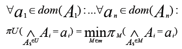
- A possibility distribution πU over U is called decomposable with respect to an undirected graph G = (U, E) if it is written as the least of the marginal possibility distributions on the maximal cliques of G, that is, if:
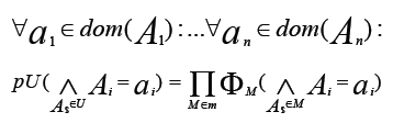
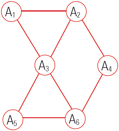
The figure represents a decomposition/factorization into four terms for an undirected graph:
These 4 terms correspond to 4 maximal cliques induced by the four sets {A1,A2,A3}, {A3,A5,A6}, {A2,A4} and {A4,A6}.
Decomposition and Directed Graphs
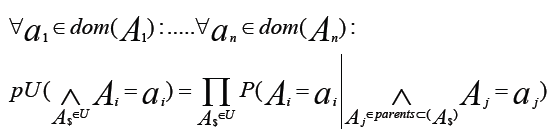
- A probability distribution pu over a set U of attributes is called. It can also call factorizable with respect to a directed acyclic graph G =(U, E). If it is written as a product of the conditional probabilities of the attributes given their parent in G, if:
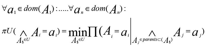
- A possibility distribution πU over U is called decomposable with respect to a directed acyclic graph G = (U, E). If it is written as the least of conditional probabilities of the attributes given their parent in G, if:
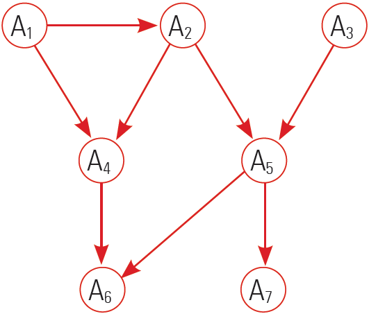
- The figure represents a decomposition/factorization into four terms for a directed graph:
Summary
We discussed the whole concept of R graphical models with its types and learned about conditional independence and decomposition in graphs.
Next, you must check the tutorial on Generalized Linear Models in R
If you have any suggestions or any query related to this R Graphical Models tutorial, ask in the comment section below.
If you are Happy with DataFlair, do not forget to make us happy with your positive feedback on Google


