Bayesian Network – Characteristics & Case Study on Queensland Railways
Job-ready Online Courses: Click, Learn, Succeed, Start Now!
The main motive of this tutorial is to provide you with a detailed description of the Bayesian Network. We will also cover Bayesian Network example and its various characteristics in R programming.
Bayesian Networks in R provide complete modeling of variables and their associated relationships. We make use of them to answer probabilistic queries.
So, let’s start the tutorial.
What is Bayesian Statistics?
Bayes’ theorem is the basis of Bayesian statistics. It enables the user to update the probabilities of unobserved events. Consider that you have a prior probability for the unobserved event and a related event has occurred. Now you can update the prior probability to get the posterior probability of the event.
Bayes’ theorem finds the posterior density of parameters for a given data. It combines information about the parameters from prior density with the observed data.
Grab a complete guide on Bayesian Networks Inference
Bayes’ Theorem – It is a theory of probability stated by the Reverend Thomas Bayes. A new piece of evidence affects the way of understanding how the probability theory holds true. We use it in a wide variety of contexts from marine biology to the development of “Bayesian” spam blockers for email systems.
When applied, the probabilities involved in Bayes’s theorem may have some probability interpretations. There is the use of the theorem as part of a particular approach to statistical inference.
What is Bayesian Network?
A Bayesian Network (BN) is a marked cyclic graph. It represents a JPD over a set of random variables V.
By using a directed graphical model, Bayesian Network describes random variables and conditional dependencies. For example, you can use a BN for a patient suffering from a particular disease. By examining various other health factors, we use BN to calculate the probability of the other related disease. Some examples are gene regular tree networks, protein structure, gene expression analysis. The following equation defines it:
B = (G, Θ)
Here:
- B is a Bayesian Network.
- G is a Directed Acyclic Graph (DAG). Its nodes X1, X2, …Xn represents random variables. Its edges represent direct dependencies between these variables. It encodes independence assumptions by which each variable Xi is independent of its non-descendants given its parents in G.
- Θ represents the set of BN parameters. This set contains the parameter Θxi |πi = PB(xi |πi for each realization of xi conditioned on π©, the set of parents of Xi in G.
B that is Bayesian Network defines a unique JPD over V, as follows:
![]()
In the above equation, for random variables xi having parents, their local probabilities distribution is conditional. The probability distribution for other variables is unconditional. Evidence nodes are the nodes that represent an observable variable whereas unseen or hidden nodes are the nodes that represent unobservable variables. For a BN, you must specify the structure and parameters for the graph model.
Conditional Probability Distribution (CPD) defines the parameters at each node and Conditional Probability Table (CPT) defines the CDP in discrete variables. Using the combination of different values from parents, CPT represents the probability of a child node.
Bayesian Network is a complete model for the variables and their relationships. We use it to answer probabilistic queries about them.
You must definitely check the tutorial on Bayesian Methods
Examples of Bayesian Network in R
Suppose you want to determine the possibility of grass getting wet or dry due to the occurrence of different seasons.
The weather has three states: Sunny, Cloudy, and Rainy. There are two possibilities for the grass: Wet or Dry.
The sprinkler can be on or off. If it is rainy, the grass gets wet but if it is sunny, we can make grass wet by pouring water from a sprinkler.
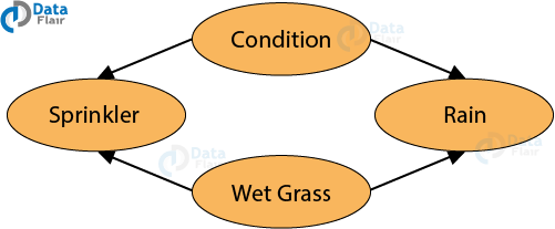
When the probabilities of the Bayesian Network reflect the weather and lawn, then the BN can answer questions such as what is the probability that rain or sprinkler makes the lawn wet? If the probability of rain increases, how will it impact the use of sprinkler to water the lawn?
Suppose that the grass is wet. This could be contributed by one of the two reasons – Firstly, it is raining. Secondly, the sprinklers are turned on. Using the Baye’s Rule, one can deduce the most contributing factor towards the wet grass which in this case is due to the rains.
Characteristics of Bayesian Networks in R
It is important to understand some characteristics associated with Bayesian Networks in R. They include the following:
- Explaining away
- Top-down and Bottom-up Reasoning
- Casualty
- Conditional Independence in BNs
- BNs with Discrete and Continuous Nodes
- Temporal Models
- Hidden Markov Models (HMMs)
- Linear Dynamic Systems (LDS) and Kalman Filters
1. Explaining Away
In the water sprinkler example, the two causes [Sprinkler (S) and Rain (R)] compete to explain the observed data. The common child ‘W’ observe that S and R become dependent, even though they are independent. This phenomenon is called explaining away because either of the two cause is adequate to explain the fact on W. In wet grass example, the grass is wet at a time and at the same time, it is raining too. It reduces the posterior probability.
2. Bottom-Up and Top-Down Reasoning
BNs are often called generative models because they specify how the causes generate effects. In the water sprinkler example, you had any evidence of an effect, which is wet grass, and you inferred the most likely cause. This approach is called bottom-up or diagnostic reasoning. It goes from effects to causes and creates a kind of inverse probability. In a BN graph, you can perform the bottom-up reasoning by going through evidence nodes connected through its descendant nodes.
Top-down or casual reasoning calculates the probability that the grass will be wet given that it is cloudy. In a BN graph, for a node X, top-down reasoning can be performed by going through the evidence nodes connected through its ancestor nodes.
3. Casualty
Casualty discussions explain the cause and effect of a phenomenon. For example – What phenomenon causes what, what are the main factors behind an effect? Previously we had to do experiments to deduce casualty in a phenomenon but BNs gives a solid mathematical foundation for casualty discussions without an experiment.
4. Conditional Independence
The Bayes Ball algorithm explains the conditional independence relationships encoded by a BN. It states that two sets of nodes A and B are independent given a set C if there is no way for a ball to move from A to B in the graph.
Don’t forget to explore the Bayesian Network Applications
5. BNs with Discrete and Continuous Nodes
The water sprinkler example used nodes with categorical values and multinomial distributions. The user can also create BNs with continuous-valued nodes. The most common distribution for these variables is Gaussian. The logistic or softmax distribution is used for discrete nodes with continuous parents. You can make complex models using multinomial, conditional Gaussian and the logistic distribution.
6. Temporal Models
By direct graphical models, Temporal models represent a process based on random inputs or variables. Temporal models are the directed graphical models of stochastic processes. They are also known as Dynamic BNs (DBNs). The simplest DBNs are Hidden Markov Models (HMM) and Linear Dynamic Systems (LDS). Temporal models simplify HMMs and LDSs by using states of variables as hidden or observed.
7. Hidden Markov Model (HMM)
An HMM that has one discrete hidden node and one discrete or continuous observed node per slice. The figure below shows an HMM:
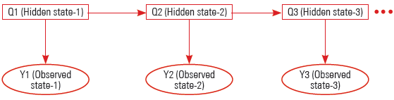
Circle symbol represents variables having continuous values. The square symbol represents variables having discrete values. Here the HMM unroll for four-time slices. Duplication of the body of a loop several times is called Unrolling. The copies are used to replace the original body. Duplication of copies is called unrolling factor.
To describe BDN, you have to express topology within and between slices. You also need to define parameters for 2 slices. Such networks with two slice temporal are also known as the 2 TBN.
8. Linear Dynamic Systems (LDSs) and Kalman Filters
An LDS has the same topology as an HMM, but it assumes to have all the nodes in linear-Gaussian distributions. A linear-Gaussian distribution is as follows:
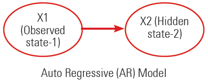
Auto Regressive Model
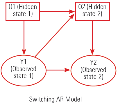
Switching AR Model
Bayesian Network – Case Study on Queensland Railways
Bayesian Networks are widely used for reasoning with uncertainty. In this, different information sources are combined to bolster intelligent support systems. Bayesian Networks closely work with the domain and therefore require the expertise of those who possess the required knowledge. In this case study, we will discuss how Bayesian Networks are being used to build customer satisfaction to bolster management decisions in transport systems.
At the Queensland Rails, Australia, customer satisfaction is a major Key Performance Indicator (KPI) that drives their business. Traditionally, Queensland Railways utilized questionnaire answering to survey the opinions of commuters. However, this proved to be ineffective to gauge the general opinion or gain insights about their services for further improvement. With the help of Bayesian Networks, they are able to meet these requirements.
The data that was used in developing the Bayesian Model consisted of questionnaires. The questions addressed were about the attributes and factors of customer service. These factors were divided into two levels of peak time and off-peak time. Furthermore, for each factor, customer responses were attributed to the category of Positive, Negative or Neutral Experiences. Factors that influenced customer experiences like Journey Components and Holistic Components.
The Journey Components were further influenced by factors like Carriage, Station Facility, Operation Information, etc. The Holistic Components were influenced by the Service Factor and Passenger Factors. Three probability states were taken to design each node – Positive, Negative and Neutral. Finally, the relationship between these models was established. The following visualization provides an example of one of the components of the model that are used to derive inferences about customer satisfaction:
After conducting the influence analysis on the model, it was concluded that the Journey Components node had a stronger influence on the Customer Satisfaction Node than the Holistic Components node. Furthermore, station components had the maximum influence on the Journey Components node. Finally, scenarios were defined by the Queensland Railways and the consequent changes in the probability of the model were observed. Some of these scenarios were – infrastructure improvement, fare increases, decreased safety, etc.
Summary
In this Bayesian Network tutorial, we discussed about Bayesian Statistics and Bayesian Networks. Moreover, we saw Bayesian Network examples and characteristics of Bayesian Network.
Now, it’s the turn of Normal Distribution in R Programming
Still, if you have any doubt, ask in the comment section.
You give me 15 seconds I promise you best tutorials
Please share your happy experience on Google


