SAS/STAT Spatial Analysis – 4 Important Procedures
Job-ready Online Courses: Click, Learn, Succeed, Start Now!
In our last tutorial, we studied SAS survival analysis Procedure. Here, we will discuss SAS/STAT Spatial Analysis. We will also learn important procedures used in Spatial Analysis in SAS/STAT: PROC KRIGE2D, PROC SIM2D, PROC SPP, and PROC VARIOGRAM with Syntax & Examples.
So, let’s start SAS/STAT Spatial Analysis.
What is SAS/STAT Spatial Analysis?
Like other processes, SAS Spatial analysis also turns raw data into useful information. The basic motive behind SAS/STAT spatial data analysis is to derive useful insights from real-world phenomena such as crimes, natural disasters, mining of ores, vegetation, and so by making use of their location and context.
You will always find spatial analysts very curious as to why things happen, how they happen, where they do. They are also curious about the effect of those phenomena on nearby regions. A spatial analysis in SAS/STAT finds its application in various fields such as agriculture, public health, insurance, forestry, crime analysis, environmental monitoring, and, energy.
Procedures for Spatial Analysis in SAS/STAT
Following procedures use to compute SAS/STAT spatial analysis of a sample data. Let us explore it.
a. PROC KRIGE2D
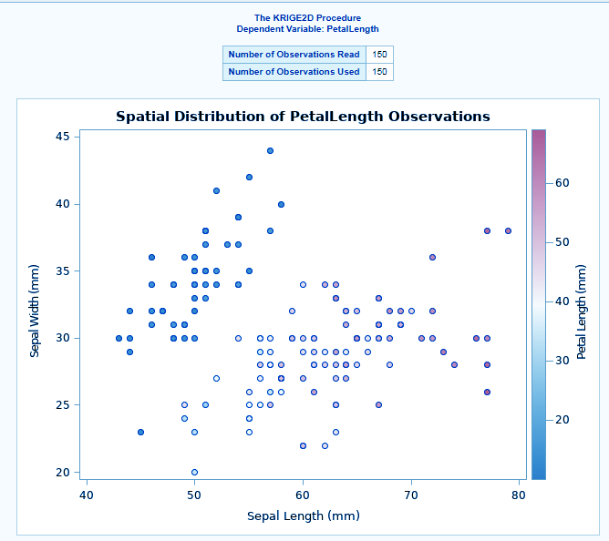
SAS PROC KRIGE2D performs spatial prediction of any spatial point reference data. The basic function is kriging, kriging is a procedure that generates estimates of a particular surface by making use of a scattered set of points that have z-values.
It has a grid statement where we specify the locations of kriging predictions. The output data set has both the kriging predictions and the standard errors associated with the data.
A Syntax of PROC KRIGE2D-
PROC krige2d DATASET<options>;
COORDINATES | COORD coordinate-variables;
GRID grid-options;
PREDICT | PRED | P predict-options;
MODEL model-options;
PROC KRIGE2D Example-
ods graphics on;
proc krige2d data=sashelp.iris plots=all;
   coordinates xcoord=sepallength ycoord=sepalwidth;
   predict var=petallength radius=60;
   model scale=7.4599 range=30.1111 form=gauss;
   grid x=0 to 100 by 2.5 y=0 to 100 by 2.5;
run;
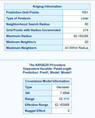
The PROC PREDICT, KRIGE2D and the MODEL statement is required and you provide the prediction parameters in the PREDICT statement.
The coordinates of the variable are specified in the COORDINATES statement.
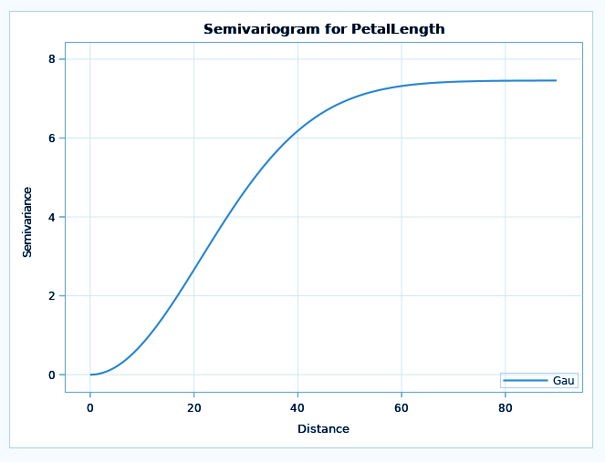
The MODEL statement contains the parameters that describe your data spatial correlation. Namely, the FORM= option specifies the model type say Gaussian, exponential etc, based on its mathematical form.
The SCALE= and RANGE=options specify the model scale on which we want the data to be analyzed and range, respectively.
The region of predictions is specified with the GRID statement.
SAS/STAT Spatial Analysis – PROC KRIGE2D
SAS/STAT Spatial Analysis – PROC KRIGE2D
SAS/STAT Spatial Analysis – PROC KRIGE2D
b. PROC SIM2D
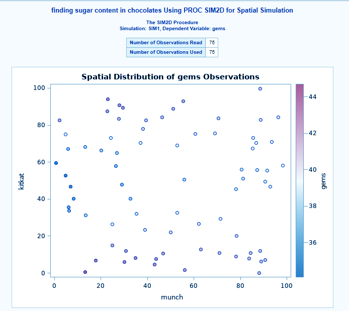
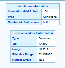
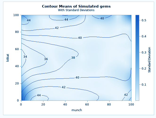
The SIM2D procedure in SAS/STAT spatial analysis also produces a spatial simulation but for a Gaussian field. It uses a decomposition technique to also specify mean and covariance structure in two dimensions. The most important feature is that it enables you to specify the covariance and the mean structure by naming the form.
The locations of the simulation points that are specified in the grid statement are also available with this procedure just like the krige2d procedure.
A Syntax of PROC SIM2D-
PROC SIM2D DATASET<options>;
SIMULATE simulate-options;
MEAN mean-options;
COORDINATES | COORD coordinate-variables;
GRID grid-options;
The PROC SIM2D and SIMULATE statement is required.
PROC SIM2D Example-
title 'finding sugar content in chocolates Using PROC SIM2D for Spatial Simulation';
data chocolates;
   input munch kitkat gems @@;
   datalines;
    0.7  59.6  34.1   2.1  82.7  42.2   4.7  75.1  39.5
    4.8  52.8  34.3   5.9  67.1  37.0   6.0  35.7  35.9
    6.4  33.7  36.4   7.0  46.7  34.6   8.2  40.1  35.4
   13.3   0.6  44.7  13.3  68.2  37.8  13.4  31.3  37.8
   17.8   6.9  43.9  20.1  66.3  37.7  22.7  87.6  42.8
   23.0  93.9  43.6  24.3  73.0  39.3  24.8  15.1  42.3
   24.8  26.3  39.7  26.4  58.0  36.9  26.9  65.0  37.8
   27.7  83.3  41.8  27.9  90.8  43.3  29.1  47.9  36.7
   29.5  89.4  43.0  30.1   6.1  43.6  30.8  12.1  42.8
   32.7  40.2  37.5  34.8   8.1  43.3  35.3  32.0  38.8
   37.0  70.3  39.2  38.2  77.9  40.7  38.9  23.3  40.5
   39.4  82.5  41.4  43.0   4.7  43.3  43.7   7.6  43.1
   46.4  84.1  41.5  46.7  10.6  42.6  49.9  22.1  40.7
   51.0  88.8  42.0  52.8  68.9  39.3  52.9  32.7  39.2
   55.5  92.9  42.2  56.0   1.6  42.7  60.6  75.2  40.1
   62.1  26.6  40.1  63.0  12.7  41.8  69.0  75.6  40.1
   70.5  83.7  40.9  70.9  11.0  41.7  71.5  29.5  39.8
   78.1  45.5  38.7  78.2   9.1  41.7  78.4  20.0  40.8
   80.5  55.9  38.7  81.1  51.0  38.6  83.8   7.9  41.6
   84.5  11.0  41.5  85.2  67.3  39.4  85.5  73.0  39.8
   86.7  70.4  39.6  87.2  55.7  38.8  88.1   0.0  41.6
   88.4  12.1  41.3  88.4  99.6  41.2  88.8  82.9  40.5
   88.9   6.2  41.5  90.6   7.0  41.5  90.7  49.6  38.9
   91.5  55.4  39.0  92.9  46.8  39.1  93.4  70.9  39.7
   55.8  50.5  38.1  96.2  84.3  40.3  98.2  58.2  39.5
;
ods graphics on;
proc sim2d data=chocolates outsim=sim plot=(observ sim);
   coordinates xc=munch yc=kitkat;
   simulate var=gems numreal=5000 seed=79931
      scale=7.4599 range=30.1111 nugget=1e-8 form=gauss;
   mean 40.1173;
   grid x=0 to 100 by 2.5 y=0 to 100 by 2.5;
run;
Spatial Analysis in SAS/STAT – PROC SIM2D
SAS PROC SIM2D
Spatial Analysis in SAS/STAT – PROC SIM2D
c. PROC SPP
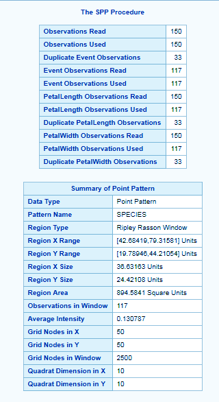
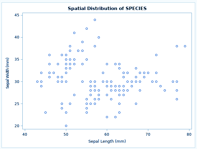
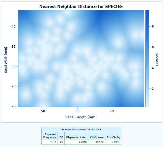
The SPP procedure in SAS/STAT describes the occurrence of observations by using spatial point pattern analysis. The observations are discrete and random, so through analysis, it characterizes the spatial process. Its unique abilities include fitting an inhomogeneous Poisson process, produce non-parametric estimates, compute correlation functions and many more. Apart from this, it also performs marked point pattern analysis.
A Syntax of PROC SPP-
PROC SPP DATASET<options>;
PROCESS name = (variables </pattern-options>)</process-options <distance-function-options>>;
TREND name = FIELD(field-definition );
The PROC SPP and PROCESS statement is required.
PROC SPP Example-
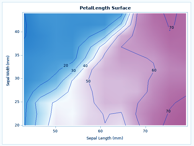
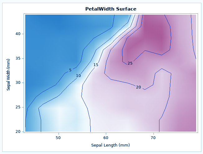
ods graphics on;
proc spp data=sashelp.IRIS plots=all;
   process SPECIES = (SEPALLENGTH, SEPALWIDTH / EVENT=SPECIES);
   trend PETALLENGTH = field(SEPALLENGTH,SEPALWIDTH, PETALLENGTH );
   trend PETALWIDTH = field(SEPALLENGTH,SEPALWIDTH, PETALWIDTH);
run;
The variables PETALLENGTH and PETALWIDTH are both continuous functions because any arbitrary point that is chosen in the study area has a value for both these variables.
In SAS/STAT spatial analysis, such CONTINUOUS variables are termed field variables and are associated with a spatial trend. They can be included in the SPP procedure by using the TREND statement. In the SPP procedure, you are required to identify the point pattern event identifier separately. This is done by using the EVENT= option in the PROCESS statement to specify that the variable SPECIES identifies the event.
SAS Spatial Analysis – PROC SPP
SAS Spatial Analysis – PROC SPP
SAS Spatial Analysis – PROC SPP
SAS Spatial Analysis – PROC SPP
SAS/STAT Spatial Analysis
d. PROC VARIOGRAM
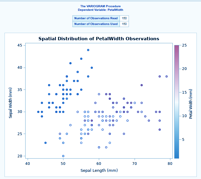
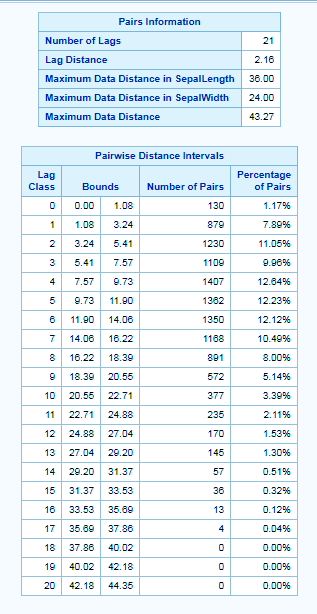
The VARIOGRAM in SAS/STAT is used to describe the spatial covariance structure in spatial point referenced data by computing variogram diagnostics. SAS VARIOGRAM procedure has the ability to fit theoretical models so that they can be used for subsequent analysis and can also handle semivariogram and anisotropic models. It makes use of eight semivariogram models such as cubic, Gaussian, exponential, spheric and so on.
A Syntax PROC VARIOGRAM-
PROC VARIOGRAM DATASET<options>;
COMPUTE computation-options;
COORDINATES coordinate-variables;
The PROC VARIOGRAM, COMPUTE, and COORDINATE statements are required.
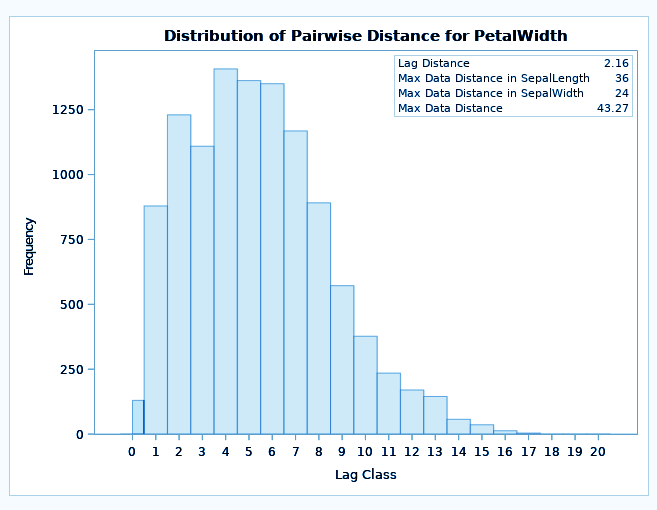
PROC VARIOGRAM Example-
ods graphics on;
proc variogram data=sashelp.IRIS plots=all;
   compute novariogram nhc=20;
   coordinates xcoord=sepallength ycoord=sepalwidth;
   var petalwidth;
run;
SAS/STAT Spatial Analysis – PROC VARIOGRAM
SAS/STAT Spatial Analysis – PROC VARIOGRAM
SAS/STAT Spatial Analysis – PROC VARIOGRAM
So, this was all about SAS/STAT Spatial Analysis Tutorial. Hope you like our explanation.
Conclusion
Hence, this was all about SAS/STAT Spatial Analysis and procedures offered by spatial analysis in SAS/STAT: PROC KRIGE2D, PROC SIM2D, PROC SPP, and PROC VARIOGRAM with Examples & Syntax. For any queries, post your doubts in the comments section below.
Your opinion matters
Please write your valuable feedback about DataFlair on Google


