4 Important SAS/STAT Longitudinal Data Analysis Procedures
FREE Online Courses: Click, Learn, Succeed, Start Now!
1. Objective
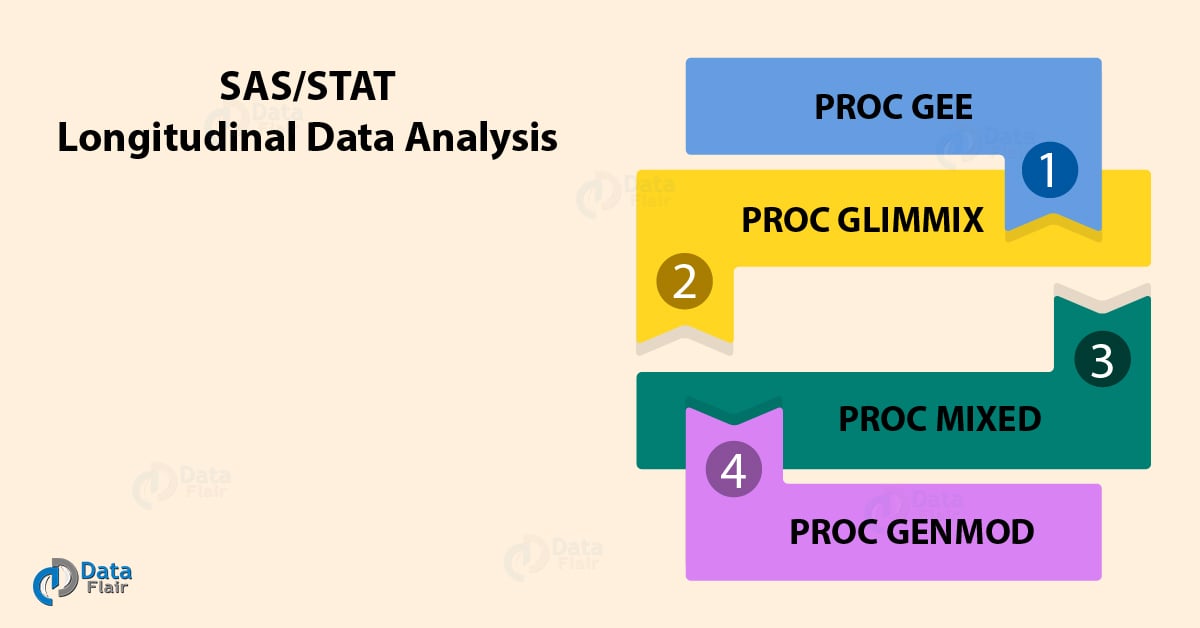
In our last tutorial, we studied SAS/STAT Exact Inference. Today we will look at SAS/STAT longitudinal data analysis. Moreover, we will see how can we use longitudinal data analysis in SAS/STAT. Our focus here will be to understand different procedures: PROC GEE, PROC GLIMMIX, PROC MIXED, PROC GENMOD that can be used for SAS/STAT longitudinal data analysis. At last, we will discuss some longitudinal analysis example.
So, let’s start with SAS/STAT Longitudinal Data Analysis.
2. SAS/ STAT Longitudinal Data Analysis
Longitudinal data arises when you measure a response variable of interest multiple numbers of times on multiple subjects. Thus, longitudinal data has the characteristics of both cross-sectional data and time-series data. The response variables in studies of longitudinal data can be either continuous or discrete.
The basic motive behind a SAS/STAT Longitudinal data analysis is usually to model the expected value of the response variable as either a linear or nonlinear function of a set of explanatory variables. Statistical analysis of longitudinal data requires an accounting for possible between-subject heterogeneity and within-subject correlation.
Let’s Revise SAS/STAT Advantages & Disadvantages
SAS/STAT software provides two approaches for modeling longitudinal data: marginal models (also known as population-average models) and mixed models (also known as subject-specific models).
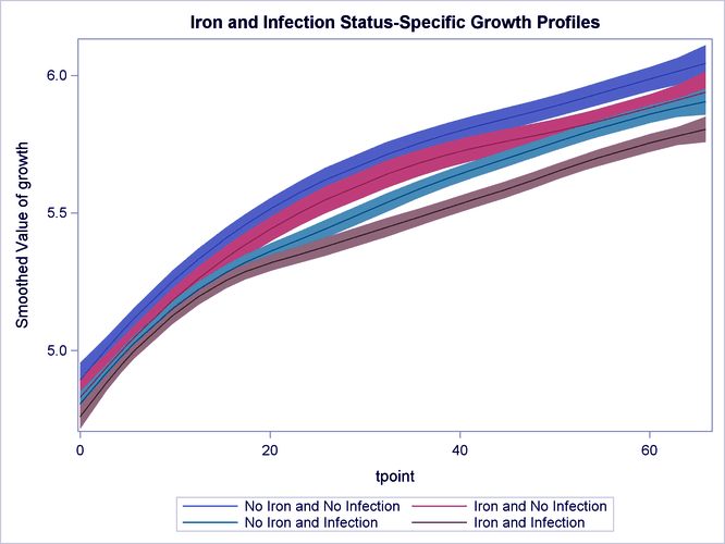
Below is a sample plot showing a SAS/STAT longitudinal data analysis representation.
3. Longitudinal Data Analysis Procedures in SAS/STAT
Following procedures use to perform SAS/STAT longitudinal data analysis of a sample data. Each procedure has a different syntax and is used with different type of data in different contexts. Let us explore each one of these.
Read About 8 Procedures for Calculating Analysis of Variance
a. PROC GEE
The PROC GEE procedure in SAS/STAT is a comprehensive tool for analyzing longitudinal data. For longitudinal studies, missing data are common, and they can be caused by dropouts or skipped visits. If missing responses depend on previous responses, the usual GEE approach can lead to biased estimates. So the GEE procedure also implements the weighted GEE method to handle missing responses that are caused by dropouts in longitudinal studies.
PROC GEE Syntax-
PROC GEE  DATASET
CLASS <variable>;
MODEL response= effects <options>;
REPEATED subject=subject effects/<options>;
The PROC GEE, MODEL, and REPEATED statements are required. All other statements can appear only once.
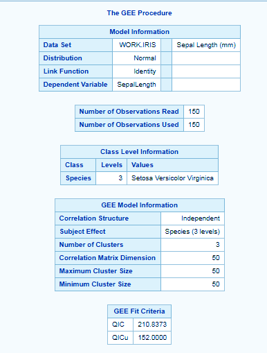
PROC GEE Example-
data iris;
set sashelp.iris;
run;
proc gee data=iris;
class species;
model sepallength=sepalwidth;
repeated subject=species;
run;
Let’s Discuss 6 SAS/STAT Bayesian Analysis Procedures
b. PROC GLIMMIX
The PROC GLIMMIX procedure in SAS/STAT performs longitudinal data analysis through which it fits statistical models to data with correlations or nonconstant variability and where the response is not necessarily normally distributed. These models are known as generalized linear mixed models (GLMM). GLMMs, like linear mixed models, assume normal (Gaussian) random effects.
PROC GLIMMIX Syntax-
PROC GLIMMIX dataset <OPTIONS>;
CLASS <VARIABLES>;
MODEL response= effects <options>;
The PROC GLIMMIX and MODEL statements are required. All other statements can appear only once.
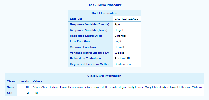
PROC GLIMMIX Example-
proc glimmix data=sashelp.class;
class name sex;
model age/height=weight/solution;
random intercept/subject=weight;
run;
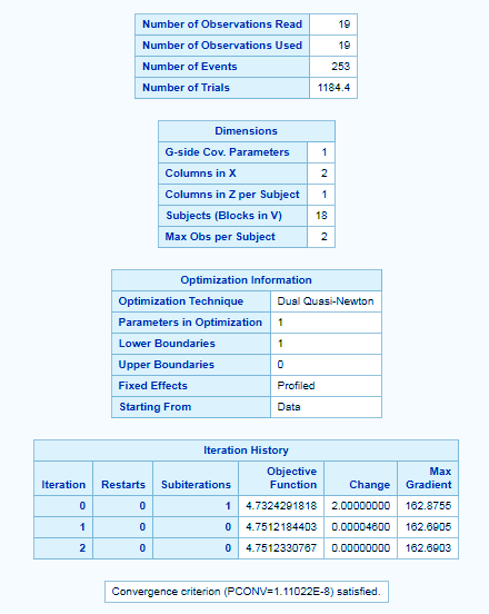
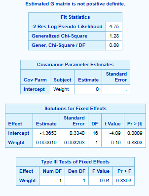
The CLASS statement instructs the procedure to treat the variables age and sex as classification variables. The MODEL statement specifies the response variable as a sample proportion by using the events/trials syntax.
The SOLUTION option in the MODEL statement requests a listing of the solutions for the fixed-effects parameter estimates.
The RANDOM statement specifies that a random intercept is drawn separately and independently for each center in the study.
Let’s Learn 7 Simple SAS/STAT Cluster Analysis Procedures
Read About SAS/STAT Group Sequential Design and Analysis
c. PROC MIXED
The PROC MIXED procedure in SAS/STAT fits different mixed models. Mixed models allow for different sources of variation in data, allows for different variances for groups and takes into account correlation structure of repeated measurements. PROC MIXED fits the structure you select to the data by using the method of restricted maximum likelihood (REML), also known as residual maximum likelihood.
PROC MIXED Syntax-
PROC MIXED dataset OPTIONS;
CLASS <VARIABLES>;
     MODEL dependent = <fixed-effects> </ options>;
The PROC MIXED and MODEL statements are required, and the MODEL statement must appear after the CLASS statement if a CLASS statement is included.
PROC MIXED Example-
ods graphics on;
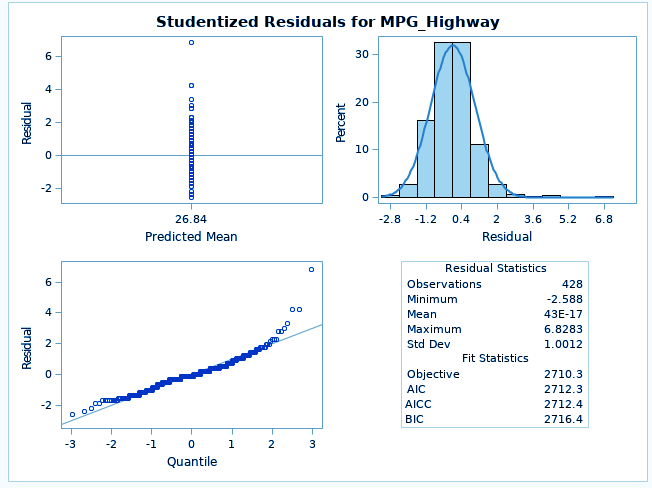
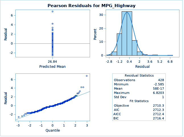
proc mixed data=SASHELP.CARS  plots=all ;
            class Origin;
            model MPG_Highway= /;
run;
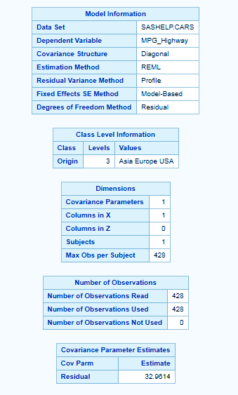
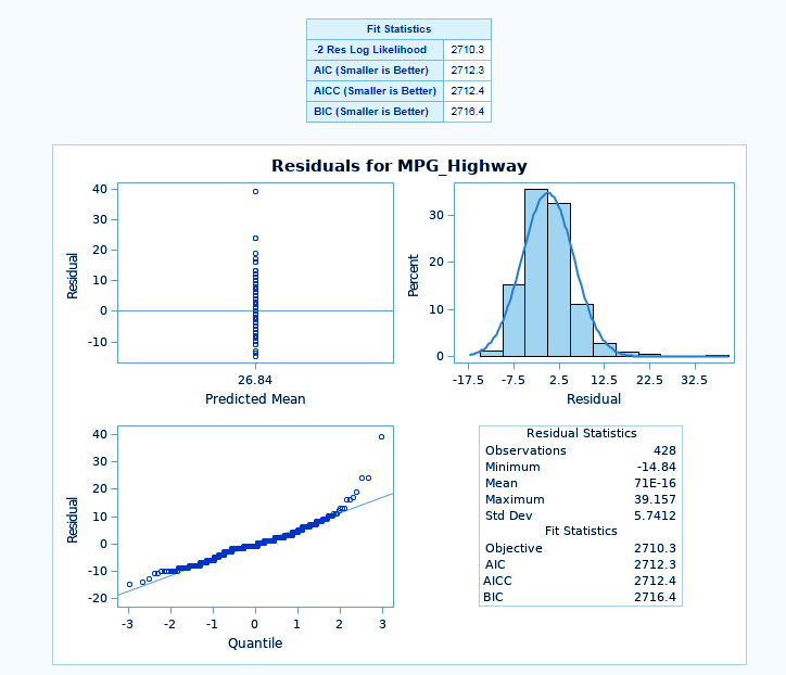
The MODEL statement first specifies the response (dependent) variable MPG_highway. The explanatory (independent) variables are then listed after the equal (=) sign. Here, no explanatory variables are used.
d. PROC GENMOD
We have already discussed this procedure in detail. You can refer to the following link for the complete tutorial.
So, This was all about SAS/STAT Longitudinal Data Analysis Tutorial. Hope you like our explanation.
4. Conclusion
Hence, this was a complete description and a comprehensive understanding of all the procedures offered by SAS/STAT longitudinal data analysis. We looked at each one of Procedures: PROC GEE, PROC GLIMMIX, PROC MIXED, and PROC GENMOD with syntax, and how they can use. Hope you all enjoyed it. Stay tuned for more interesting topics in SAS/STAT, and for any doubts, post it in the comments section below.
Related Topic- SAS/STAT Categorical Data Analysis Procedure
Did you like our efforts? If Yes, please give DataFlair 5 Stars on Google



Great doing it