SAS/STAT Distribution Analysis – KDE Procedure
Placement-ready Courses: Enroll Now, Thank us Later!
In our last SAS/STAT tutorial, we studied STAT Group Sequential Design and Analysis. Today, we will be looking at another type of analysis called SAS/STAT distribution analysis. Moreover, we will also discuss how distribution analysis is used in SAS/STAT for kernel density estimation.
Our focus here will be to understand the KDE procedure that can be used for SAS/STAT Distribution analysis through the use of an example.
So, let’s start with SAS/STAT Distribution Analysis.
SAS/STAT Distribution Analysis
The distribution of a statistical data set is a listing or function showing all the possible values of the data and how often they occur. When a distribution of categorical data is organized, you see the number or percentage of individuals in each group.
When a distribution of numerical data is organized, they’re often ordered from smallest to largest, broken into reasonably sized groups, and then put into graphs and charts to examine the shape, centre, and amount of variability in the data.
SAS/STAT Distribution analysis provides information about the distribution of numeric variables. A variety of plots such as histograms, probability plots, and quantile-quantile plots can be used in this analysis.
Example of Distribution Analysis in SAS/STAT
Procedures for Distribution Analysis in SAS/STAT
Following procedure is used to compute SAS/STAT distribution analysis of a sample data. Let’s explore each of it.
a. PROC KDE
The PROC KDE procedure in SAS/STAT performs univariate and multivariate estimation. The kernel density estimation technique is a technique used for density estimation in which a known density function, known as a kernel, is averaged across the data to create an approximation. It is very similar to the way we plot a histogram.
PROC KDE Syntax-
PROC KDE DATASET;
Univar <variables>;
Bivar <variables>;
data bivar;
   seed = 1234567;
   do i = 1 to 1000;
      z1 = rannor(seed);
      z2 = rannor(seed);
      z3 = rannor(seed);
      x = 3*z1+z2;
      y = 3*z1+z3;
      output;
   end;
   drop seed;
run;
/**kernel density plot**/
ods graphics on;
proc kde data=bivar;
   univar x ;
run;
/**bivariate plot**/
ods graphics on;
proc kde data=bivar;
   bivar x y / plots=all;
run;
ods graphics off;
The UNIVAR statement computes one or more univariate kernel density estimates and similarly, the BIVAR statement computes bivariate kernel density estimate.
The PLOTS= option prints different plots between the two variables. We can specify the type of plot we want inside the brackets, we have displayed all plots here.
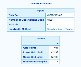
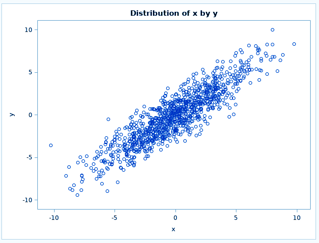
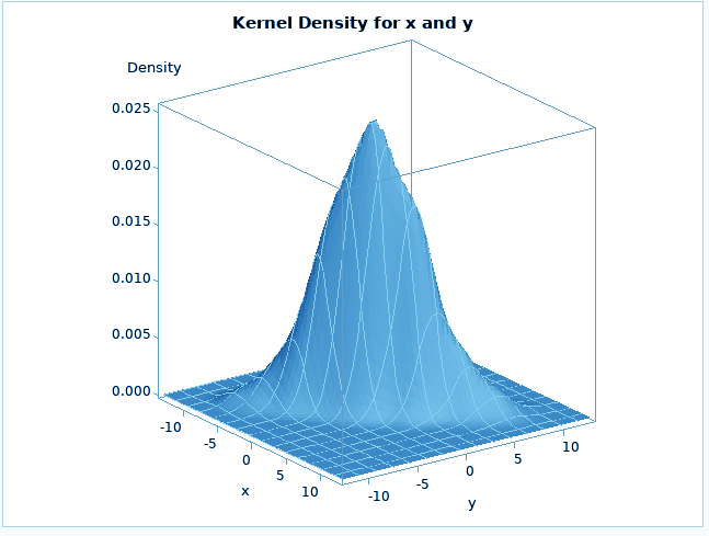
Distribution Analysis in SAS/STAT – PROC KDE
Distribution Analysis in SAS/STAT – PROC KDE
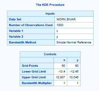
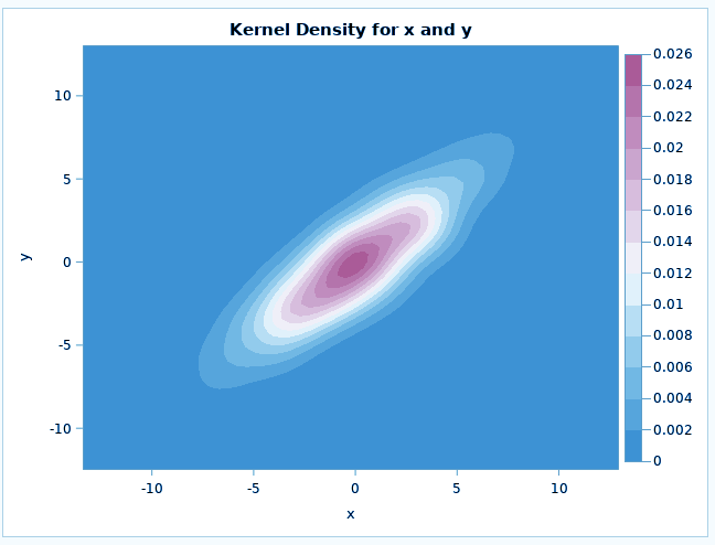
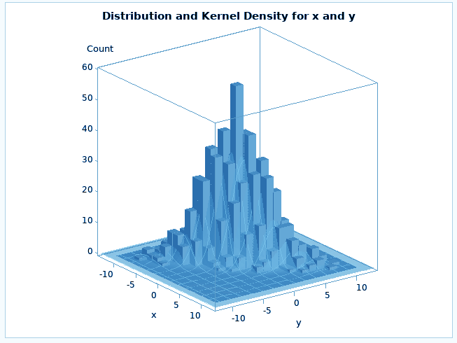
SAS/STAT Distribution Analysis
Distribution Analysis in STAT – PROC KDE
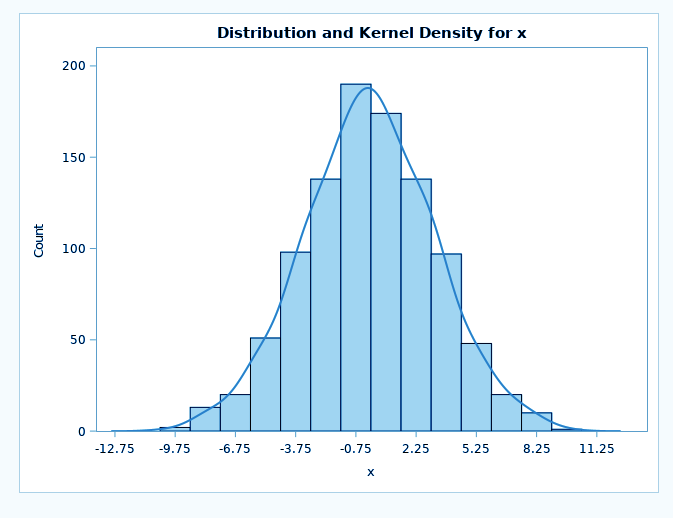
Distribution Analysis in SAS – PROC KDE
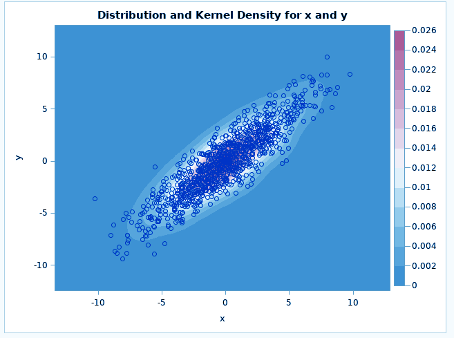
Distribution Analysis in SAS – PROC KDE
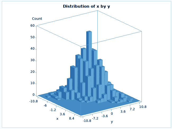
SAS/STAT Distribution Analysis – PROC KDE
SAS/STAT Distribution Analysis – PROC KDE
SAS/STAT Distribution Analysis – PROC KDE
Hence, this was all about SAS/STAT Distribution Analysis. Hope you like our explanation.
Conclusion
So finally, this was a complete description and a comprehensive understanding of the KDE procedure offered by SAS/STAT distribution analysis. Stay tuned for more interesting topics in SAS/ STAT. Furthermore, for any queries, post your doubts in the comments section below.
If you are Happy with DataFlair, do not forget to make us happy with your positive feedback on Google


