SAS Histogram Statement with UNIVARIATE Procedure & Normal Curve

The most important aspect of data analysis is a representation of data in the form of graphs and charts. Today we will be looking at how to represent our data in the form of a histogram in SAS Programming Language.

Besides this, we will also be looking at the different functions and parameters that can be added to our SAS histogram to make it easier to understand. We will also study PROC univariate histogram normal curve.

Let’s start with SAS Histogram Statements.

What is SAS Histogram?

In statistics, a histogram is a graphical display of tabulated frequency. SAS histogram differs from a bar chart in that it is the area of the bar that denotes the value, not the height.

Histograms in SAS allow you to explore your data by displaying the distribution of a continuous variable (percentage of a sample) against categories of the value.

You can obtain the shape of the distribution and the data are distributed symmetrically. In SAS, the histograms can be produced using PROC UNIVARIATE, PROC CHART, or PROC GCHART. 

SAS UNIVARIATE Procedure

The syntax of creating a SAS histogram-

PROC UNIVARIATE DATA = DATASET;
HISTOGRAM variables  / options;
RUN;

With the use of SAS Histogram statement in PROC UNIVARIATE, we can have a fast and simple way to review the overall distribution of a quantitative variable in a graphical display.

You can use any number of Histogram statements in SAS after a PROC UNIVARIATE statement. The components of the SAS HISTOGRAM statement are:

1. Variables

This is used to create SAS histograms. If you do not specify variables in a VAR statement or in the HISTOGRAM statement, then by default, a histogram is created for each numeric variable in the DATA= data set.

If you use a VAR statement and do not specify any variables in the HISTOGRAM statement, then by default, a histogram is created for each variable listed in the VAR statement.

For example, suppose a data set named Steel contains exactly two numeric variables named Length and Width. The following statements create two histograms, one for Length and one for Width:

proc univariate data=Steel;
   histogram;
run;

Likewise, the following statements create histograms for Length and Width:

proc univariate data=Steel;
   var Length Width;
   histogram;
run;

The following statements create a histogram for Length only:

proc univariate data=Steel;
   var Length Width;
   histogram Length;
run;

2. Options

It adds features to the histogram. Specify all options after the slash (/) in the SAS HISTOGRAM statement.

For example, in the following statements, the NORMAL option displays a fitted normal curve on the histogram, the MIDPOINTS= option specifies midpoints for the histogram, and the CTEXT= option specifies the color of the text:

proc univariate data=Steel;
   histogram Length / normal
                      midpoints = 5.6 5.8 6.0 6.2 6.4
                      ctext     = blue;
run;

SAS Histogram with Normal Curve

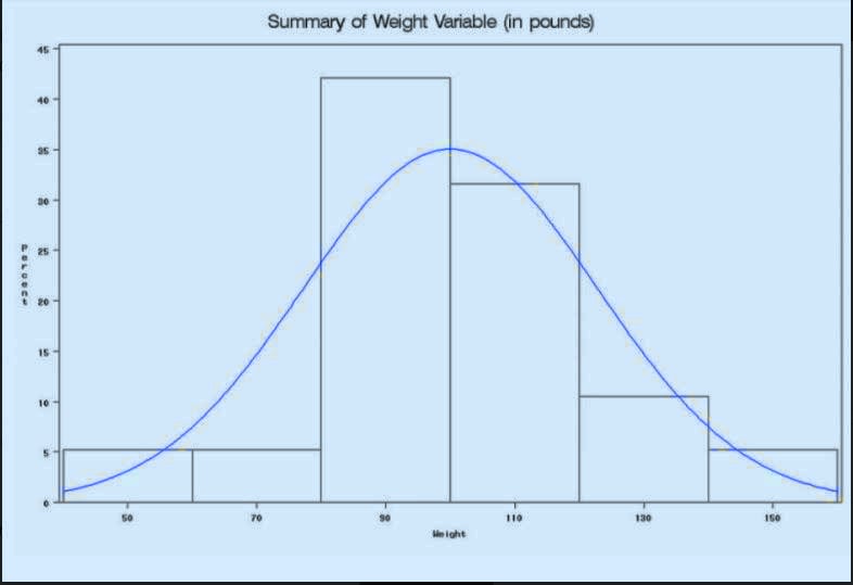
Let’s start by creating a simple SAS histogram of the WEIGHT variable. We will use the inbuilt data set sashelp.class:

TITLE 'Summary of Weight Variable (in pounds)';
 PROC UNIVARIATE DATA = sashelp.class NOPRINT;
HISTOGRAM weight / NORMAL; RUN;

We can have more than one analysis variable in the SAS Histogram statement. Each variable will have a separate histogram in SAS. NOPRINT option suppresses the summary statistics, the NORMAL option presents a normal curve.

SAS Histogram with Different Customizable Options

With the SAS histogram statement, different options can be added to the following:

1. We can add the CFILL option to fill color for the histogram and INSET statement to insert a box of the summary statistics directly in the graph.

2. By default the font of the text in the inset bo inside the graph is FONT=SIMPLEX.

3. The MIDPOINTS= option specifies midpoints for the histogram,

4. The CTEXT= option specifies the color of the text.

Example-

PROC UNIVARIATE DATA = sashelp.class;
HISTOGRAM weight / NORMAL CFILL = ltgray;
INSET N = 'Number of students' MEDIAN (8.2) MEAN (8.2) STD=’Standard Deviation’ (8.3) / POSITION = ne;
RUN;

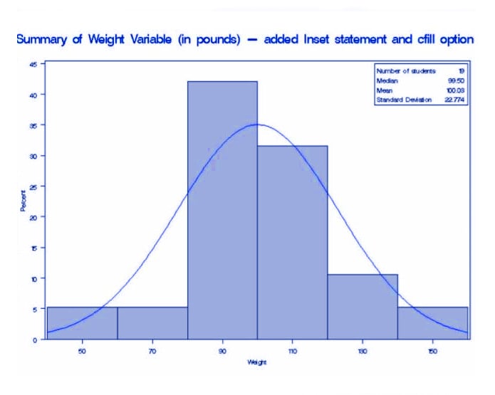
The above graph shows the SAS histogram with different customizable options

Summary

We saw two ways to design SAS histogram, one was a basic one, the other was with different options to suit our requirements. SAS has a repository of text styles, colors, options that can be added to our histogram for better readability. You can go through them in the SAS help directory.

If you have any query feel free to ask in the comment section.