Introduction to Learning Rules in Neural Network

1. Objective

Learning rule is a method or a mathematical logic. It helps a Neural Network to learn from the existing conditions and improve its performance. It is an iterative process. In this machine learning tutorial, we are going to discuss the learning rules in Neural Network. What is Hebbian learning rule, Perceptron learning rule, Delta learning rule, Correlation learning rule, Outstar learning rule? All these Neural Network Learning Rules are in this tutorial in detail, along with their mathematical formulas.

Introduction to Learning Rules in Neural Network

2. What are the Learning Rules in Neural Network?

Learning rule or Learning process is a method or a mathematical logic. It improves the Artificial Neural Network’s performance and applies this rule over the network. Thus learning rules updates the weights and bias levels of a network when a network simulates in a specific data environment.
Applying learning rule is an iterative process. It helps a neural network to learn from the existing conditions and improve its performance.
Let us see different learning rules in the Neural network:

• Hebbian learning rule – It identifies, how to modify the weights of nodes of a network.
• Perceptron learning rule – Network starts its learning by assigning a random value to each weight.
• Delta learning rule – Modification in sympatric weight of a node is equal to the multiplication of error and the input.
• Correlation learning rule – The correlation rule is the supervised learning.
• Outstar learning rule – We can use it when it assumes that nodes or neurons in a network arranged in a layer.

2.1. Hebbian Learning Rule

The Hebbian rule was the first learning rule. In 1949 Donald Hebb developed it as learning algorithm of the unsupervised neural network. We can use it to identify how to improve the weights of nodes of a network.
The Hebb learning rule assumes that – If two neighbor neurons activated and deactivated at the same time. Then the weight connecting these neurons should increase. For neurons operating in the opposite phase, the weight between them should decrease. If there is no signal correlation, the weight should not change.
When inputs of both the nodes are either positive or negative, then a strong positive weight exists between the nodes. If the input of a node is positive and negative for other, a strong negative weight exists between the nodes.
At the start, values of all weights are set to zero. This learning rule can be used0 for both soft- and hard-activation functions. Since desired responses of neurons are not used in the learning procedure, this is the unsupervised learning rule. The absolute values of the weights are usually proportional to the learning time, which is undesired.

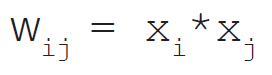
Mathematical Formula of Hebb Learning Rule in Artificial Neural Network.

The Hebbian learning rule describes the formula as follows:

2.2. Perceptron Learning Rule

As you know, each connection in a neural network has an associated weight, which changes in the course of learning. According to it, an example of supervised learning, the network starts its learning by assigning a random value to each weight.
Calculate the output value on the basis of a set of records for which we can know the expected output value. This is the learning sample that indicates the entire definition. As a result, it is called a learning sample.
The network then compares the calculated output value with the expected value. Next calculates an error function ∈, which can be the sum of squares of the errors occurring for each individual in the learning sample.
Computed as follows:

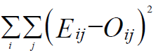
Mathematical Formula of Perceptron Learning Rule in Artificial Neural Network.

Perform the first summation on the individuals of the learning set, and perform the second summation on the output units. Eij and Oij are the expected and obtained values of the jth unit for the ith individual.
The network then adjusts the weights of the different units, checking each time to see if the error function has increased or decreased. As in a conventional regression, this is a matter of solving a problem of least squares.
Since assigning the weights of nodes according to users, it is an example of supervised learning.

2.3. Delta Learning Rule

Developed by Widrow and Hoff, the delta rule, is one of the most common learning rules. It depends on supervised learning.
This rule states that the modification in sympatric weight of a node is equal to the multiplication of error and the input.
In Mathematical form the delta rule is as follows:

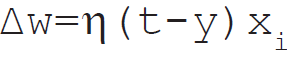
Mathematical Formula of Delta Learning Rule in Artificial Neural Network.

For a given input vector, compare the output vector is the correct answer. If the difference is zero, no learning takes place; otherwise, adjusts its weights to reduce this difference. The change in weight from ui to uj is: dwij = r* ai * ej.
where r is the learning rate, ai represents the activation of ui and ej is the difference between the expected output and the actual output of uj. If the set of input patterns form an independent set then learn arbitrary associations using the delta rule.
It has seen that for networks with linear activation functions and with no hidden units. The error squared vs. the weight graph is a paraboloid in n-space. Since the proportionality constant is negative, the graph of such a function is concave upward and has the least value. The vertex of this paraboloid represents the point where it reduces the error. The weight vector corresponding to this point is then the ideal weight vector.
We can use the delta learning rule with both single output unit and several output units.
While applying the delta rule assume that the error can be directly measured.
The aim of applying the delta rule is to reduce the difference between the actual and expected output that is the error.

2.4. Correlation Learning Rule

The correlation learning rule based on a similar principle as the Hebbian learning rule. It assumes that weights between responding neurons should be more positive, and weights between neurons with opposite reaction should be more negative.

Contrary to the Hebbian rule, the correlation rule is the supervised learning. Instead of an actual
The response, oj, the desired response, dj, uses for the weight-change calculation.
In Mathematical form the correlation learning rule is as follows:

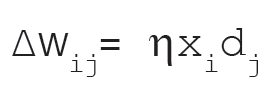
Mathematical Formula of Correlation Learning Rule in Artificial Neural Network.

Where dj is the desired value of output signal. This training algorithm usually starts with the initialization of weights to zero.
Since assigning the desired weight by users, the correlation learning rule is an example of supervised learning.

2.5. Out Star Learning Rule

We use the Out Star Learning Rule when we assume that nodes or neurons in a network arranged in a layer. Here the weights connected to a certain node should be equal to the desired outputs for the neurons connected through those weights. The out start rule produces the desired response t for the layer of n nodes.

Apply this type of learning for all nodes in a particular layer. Update the weights for nodes are as in Kohonen neural networks.
In Mathematical form, express the out star learning as follows:

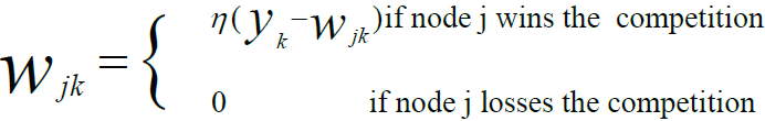
Mathematical Formula of Out Star Learning Rule in Artificial Neural Network.

This is a supervised training procedure because desired outputs must be known.

3. Conclusion

In conclusion to the learning rules in Neural Network, we can say that the most promising feature of the Artificial Neural Network is its ability to learn. The learning process of brain alters its neural structure. The increasing or decreasing the strength of its synaptic connections depending on their activity. The more relevant information has a stronger synaptic connection. Hence, there are several algorithms for training artificial neural networks with their own pros and cons.
If you feel any queries about Learning Rules in Neural network, feel free to share with us.
See Also-

• Applications of Machine Learning
• Applications of Artificial Neural Network

Reference – Machine Learning