Stock Price Prediction – Machine Learning Project in Python
Machine Learning courses with 100+ Real-time projects Start Now!!
Machine learning has significant applications in the stock price prediction. In this machine learning project, we will be talking about predicting the returns on stocks. This is a very complex task and has uncertainties. We will develop this project into two parts:
1. First, we will learn how to predict stock price using the LSTM neural network.
2. Then we will build a dashboard using Plotly dash for stock analysis.
Stock Price Prediction Project
Datasets
1. To build the stock price prediction model, we will use the NSE TATA GLOBAL dataset. This is a dataset of Tata Beverages from Tata Global Beverages Limited, National Stock Exchange of India: Tata Global Dataset
2. To develop the dashboard for stock analysis we will use another stock dataset with multiple stocks like Apple, Microsoft, Facebook: Stocks Dataset
Source Code
Before proceeding ahead, please download the source code: Stock Price Prediction Project
Stock price prediction using LSTM
1. Imports:
import pandas as pd
import numpy as np

import matplotlib.pyplot as plt
%matplotlib inline

from matplotlib.pylab import rcParams
rcParams['figure.figsize']=20,10
from keras.models import Sequential
from keras.layers import LSTM,Dropout,Dense


from sklearn.preprocessing import MinMaxScaler
2. Read the dataset:
df=pd.read_csv("NSE-TATA.csv")
df.head()
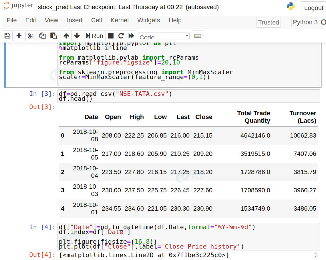
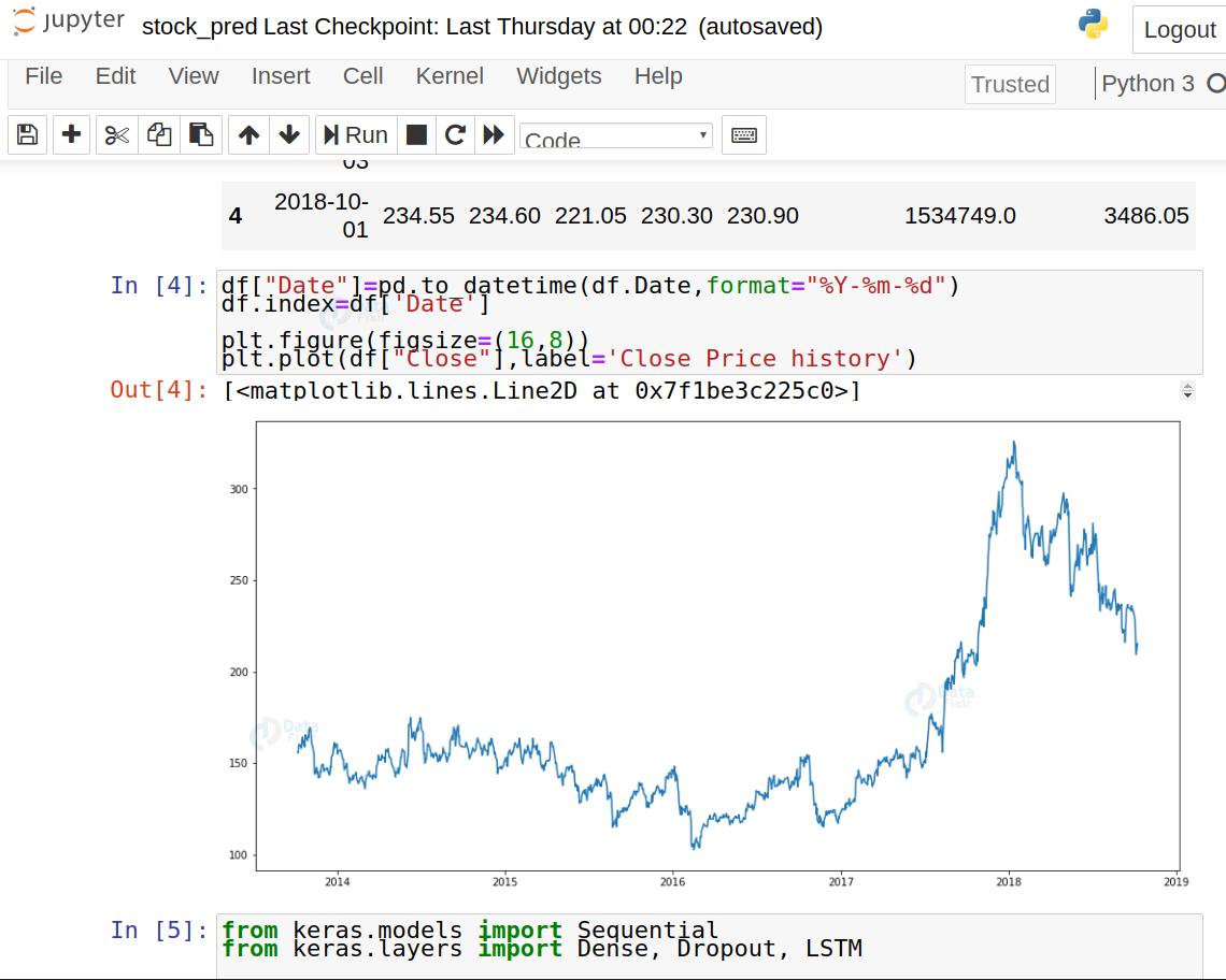
3. Analyze the closing prices from dataframe:
df["Date"]=pd.to_datetime(df.Date,format="%Y-%m-%d")
df.index=df['Date']

plt.figure(figsize=(16,8))
plt.plot(df["Close"],label='Close Price history')
4. Sort the dataset on date time and filter “Date” and “Close” columns:
data=df.sort_index(ascending=True,axis=0)
new_dataset=pd.DataFrame(index=range(0,len(df)),columns=['Date','Close'])

for i in range(0,len(data)):
    new_dataset["Date"][i]=data['Date'][i]
    new_dataset["Close"][i]=data["Close"][i]
5. Normalize the new filtered dataset:
scaler=MinMaxScaler(feature_range=(0,1))
final_dataset=new_dataset.values

train_data=final_dataset[0:987,:]
valid_data=final_dataset[987:,:]

new_dataset.index=new_dataset.Date
new_dataset.drop("Date",axis=1,inplace=True)
scaler=MinMaxScaler(feature_range=(0,1))
scaled_data=scaler.fit_transform(final_dataset)

x_train_data,y_train_data=[],[]

for i in range(60,len(train_data)):
    x_train_data.append(scaled_data[i-60:i,0])
    y_train_data.append(scaled_data[i,0])

x_train_data,y_train_data=np.array(x_train_data),np.array(y_train_data)

x_train_data=np.reshape(x_train_data,(x_train_data.shape[0],x_train_data.shape[1],1))
6. Build and train the LSTM model:
lstm_model=Sequential()
lstm_model.add(LSTM(units=50,return_sequences=True,input_shape=(x_train_data.shape[1],1)))
lstm_model.add(LSTM(units=50))
lstm_model.add(Dense(1))

inputs_data=new_dataset[len(new_dataset)-len(valid_data)-60:].values
inputs_data=inputs_data.reshape(-1,1)
inputs_data=scaler.transform(inputs_data)

lstm_model.compile(loss='mean_squared_error',optimizer='adam')
lstm_model.fit(x_train_data,y_train_data,epochs=1,batch_size=1,verbose=2)
7. Take a sample of a dataset to make stock price predictions using the LSTM model:
X_test=[]
for i in range(60,inputs_data.shape[0]):
    X_test.append(inputs_data[i-60:i,0])
X_test=np.array(X_test)

X_test=np.reshape(X_test,(X_test.shape[0],X_test.shape[1],1))
predicted_closing_price=lstm_model.predict(X_test)
predicted_closing_price=scaler.inverse_transform(predicted_closing_price)
8. Save the LSTM model:
lstm_model.save("saved_model.h5")9. Visualize the predicted stock costs with actual stock costs:
train_data=new_dataset[:987]
valid_data=new_dataset[987:]
valid_data['Predictions']=predicted_closing_price
plt.plot(train_data["Close"])
plt.plot(valid_data[['Close',"Predictions"]])
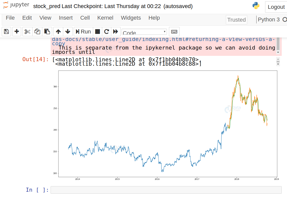
You can observe that LSTM has predicted stocks almost similar to actual stocks.
Build the dashboard using Plotly dash
In this section, we will build a dashboard to analyze stocks. Dash is a python framework that provides an abstraction over flask and react.js to build analytical web applications.
Before moving ahead, you need to install dash. Run the below command in the terminal.
pip3 install dash
pip3 install dash-html-components
pip3 install dash-core-components
Now make a new python file stock_app.py and paste the below script:
import dash
import dash_core_components as dcc
import dash_html_components as html
import pandas as pd
import plotly.graph_objs as go
from dash.dependencies import Input, Output
from keras.models import load_model
from sklearn.preprocessing import MinMaxScaler
import numpy as np


app = dash.Dash()
server = app.server

scaler=MinMaxScaler(feature_range=(0,1))

df_nse = pd.read_csv("./NSE-TATA.csv")

df_nse["Date"]=pd.to_datetime(df_nse.Date,format="%Y-%m-%d")
df_nse.index=df_nse['Date']


data=df_nse.sort_index(ascending=True,axis=0)
new_data=pd.DataFrame(index=range(0,len(df_nse)),columns=['Date','Close'])

for i in range(0,len(data)):
    new_data["Date"][i]=data['Date'][i]
    new_data["Close"][i]=data["Close"][i]

new_data.index=new_data.Date
new_data.drop("Date",axis=1,inplace=True)

dataset=new_data.values

train=dataset[0:987,:]
valid=dataset[987:,:]

scaler=MinMaxScaler(feature_range=(0,1))
scaled_data=scaler.fit_transform(dataset)

x_train,y_train=[],[]

for i in range(60,len(train)):
    x_train.append(scaled_data[i-60:i,0])
    y_train.append(scaled_data[i,0])

x_train,y_train=np.array(x_train),np.array(y_train)

x_train=np.reshape(x_train,(x_train.shape[0],x_train.shape[1],1))

model=load_model("saved_model.h5")

inputs=new_data[len(new_data)-len(valid)-60:].values
inputs=inputs.reshape(-1,1)
inputs=scaler.transform(inputs)

X_test=[]
for i in range(60,inputs.shape[0]):
    X_test.append(inputs[i-60:i,0])
X_test=np.array(X_test)

X_test=np.reshape(X_test,(X_test.shape[0],X_test.shape[1],1))
closing_price=model.predict(X_test)
closing_price=scaler.inverse_transform(closing_price)

train=new_data[:987]
valid=new_data[987:]
valid['Predictions']=closing_price


df= pd.read_csv("./stock_data.csv")

app.layout = html.Div([

    html.H1("Stock Price Analysis Dashboard", style={"textAlign": "center"}),

    dcc.Tabs(id="tabs", children=[

        dcc.Tab(label='NSE-TATAGLOBAL Stock Data',children=[
            html.Div([
                html.H2("Actual closing price",style={"textAlign": "center"}),
                dcc.Graph(
                    id="Actual Data",
                    figure={
                        "data":[
                            go.Scatter(
                                x=train.index,
                                y=valid["Close"],
                                mode='markers'
                            )

                        ],
                        "layout":go.Layout(
                            title='scatter plot',
                            xaxis={'title':'Date'},
                            yaxis={'title':'Closing Rate'}
                        )
                    }

                ),
                html.H2("LSTM Predicted closing price",style={"textAlign": "center"}),
                dcc.Graph(
                    id="Predicted Data",
                    figure={
                        "data":[
                            go.Scatter(
                                x=valid.index,
                                y=valid["Predictions"],
                                mode='markers'
                            )

                        ],
                        "layout":go.Layout(
                            title='scatter plot',
                            xaxis={'title':'Date'},
                            yaxis={'title':'Closing Rate'}
                        )
                    }

                )
            ])


        ]),
        dcc.Tab(label='Facebook Stock Data', children=[
            html.Div([
                html.H1("Facebook Stocks High vs Lows",
                        style={'textAlign': 'center'}),

                dcc.Dropdown(id='my-dropdown',
                             options=[{'label': 'Tesla', 'value': 'TSLA'},
                                      {'label': 'Apple','value': 'AAPL'},
                                      {'label': 'Facebook', 'value': 'FB'},
                                      {'label': 'Microsoft','value': 'MSFT'}],
                             multi=True,value=['FB'],
                             style={"display": "block", "margin-left": "auto",
                                    "margin-right": "auto", "width": "60%"}),
                dcc.Graph(id='highlow'),
                html.H1("Facebook Market Volume", style={'textAlign': 'center'}),

                dcc.Dropdown(id='my-dropdown2',
                             options=[{'label': 'Tesla', 'value': 'TSLA'},
                                      {'label': 'Apple','value': 'AAPL'},
                                      {'label': 'Facebook', 'value': 'FB'},
                                      {'label': 'Microsoft','value': 'MSFT'}],
                             multi=True,value=['FB'],
                             style={"display": "block", "margin-left": "auto",
                                    "margin-right": "auto", "width": "60%"}),
                dcc.Graph(id='volume')
            ], className="container"),
        ])


    ])
])


@app.callback(Output('highlow', 'figure'),
              [Input('my-dropdown', 'value')])
def update_graph(selected_dropdown):
    dropdown = {"TSLA": "Tesla","AAPL": "Apple","FB": "Facebook","MSFT": "Microsoft",}
    trace1 = []
    trace2 = []
    for stock in selected_dropdown:
        trace1.append(
          go.Scatter(x=df[df["Stock"] == stock]["Date"],
                     y=df[df["Stock"] == stock]["High"],
                     mode='lines', opacity=0.7,
                     name=f'High {dropdown[stock]}',textposition='bottom center'))
        trace2.append(
          go.Scatter(x=df[df["Stock"] == stock]["Date"],
                     y=df[df["Stock"] == stock]["Low"],
                     mode='lines', opacity=0.6,
                     name=f'Low {dropdown[stock]}',textposition='bottom center'))
    traces = [trace1, trace2]
    data = [val for sublist in traces for val in sublist]
    figure = {'data': data,
              'layout': go.Layout(colorway=["#5E0DAC", '#FF4F00', '#375CB1',
                                            '#FF7400', '#FFF400', '#FF0056'],
            height=600,
            title=f"High and Low Prices for {', '.join(str(dropdown[i]) for i in selected_dropdown)} Over Time",
            xaxis={"title":"Date",
                   'rangeselector': {'buttons': list([{'count': 1, 'label': '1M',
                                                       'step': 'month',
                                                       'stepmode': 'backward'},
                                                      {'count': 6, 'label': '6M',
                                                       'step': 'month',
                                                       'stepmode': 'backward'},
                                                      {'step': 'all'}])},
                   'rangeslider': {'visible': True}, 'type': 'date'},
             yaxis={"title":"Price (USD)"})}
    return figure


@app.callback(Output('volume', 'figure'),
              [Input('my-dropdown2', 'value')])
def update_graph(selected_dropdown_value):
    dropdown = {"TSLA": "Tesla","AAPL": "Apple","FB": "Facebook","MSFT": "Microsoft",}
    trace1 = []
    for stock in selected_dropdown_value:
        trace1.append(
          go.Scatter(x=df[df["Stock"] == stock]["Date"],
                     y=df[df["Stock"] == stock]["Volume"],
                     mode='lines', opacity=0.7,
                     name=f'Volume {dropdown[stock]}', textposition='bottom center'))
    traces = [trace1]
    data = [val for sublist in traces for val in sublist]
    figure = {'data': data,
              'layout': go.Layout(colorway=["#5E0DAC", '#FF4F00', '#375CB1',
                                            '#FF7400', '#FFF400', '#FF0056'],
            height=600,
            title=f"Market Volume for {', '.join(str(dropdown[i]) for i in selected_dropdown_value)} Over Time",
            xaxis={"title":"Date",
                   'rangeselector': {'buttons': list([{'count': 1, 'label': '1M',
                                                       'step': 'month',
                                                       'stepmode': 'backward'},
                                                      {'count': 6, 'label': '6M',
                                                       'step': 'month',
                                                       'stepmode': 'backward'},
                                                      {'step': 'all'}])},
                   'rangeslider': {'visible': True}, 'type': 'date'},
             yaxis={"title":"Transactions Volume"})}
    return figure


if __name__=='__main__':
    app.run_server(debug=True)
Now run this file and open the app in the browser:
python3 stock_app.py
Summary
Stock price prediction helps investors make smart decisions. In this project, we use Python and machine learning to predict the future price of a company’s stock. We use past stock data to train a regression model. It’s a great mix of data analysis, finance, and ML.
Stock price prediction is a machine learning project for beginners; in this tutorial we learned how to develop a stock cost prediction model and how to build an interactive dashboard for stock analysis. We implemented stock market prediction using the LSTM model. OTOH, Plotly dash python framework for building dashboards.
This project is ideal for those interested in finance and ML. It teaches time series forecasting, data visualization, model training, and evaluation. You can build a simple web app or dashboard to show predictions in real-time.
Did you like this article? If Yes, please give DataFlair 5 Stars on Google


NotImplementedError: Cannot convert a symbolic Tensor (lstm/strided_slice:0) to a numpy array. This error may indicate that you’re trying to pass a Tensor to a NumPy call, which is not supported
please help me slove this
lstm_model.add(LSTM(units=50,return_sequences=True,input_shape=(x_train_data.shape[1],1)))
NotImplementedError: Cannot convert a symbolic Tensor (lstm_4/strided_slice:0) to a numpy array. This error may indicate that you’re trying to pass a Tensor to a NumPy call, which is not supported
at this line an error is occured please help me to slove this
pycharm i s not supporting to download all these libraries involved in code…can someone help me to execute this code
Try to install all libraries in jupiter like this
!pip install name_library
Hi I am new to programming. I have downloaded the source code. But there are 2 .py files. How do I run both of them together?
Hi, could you help me with the code to take out test accuracy. I have tried but failed. Pls help.
Can anyone provide me with the dataset that they used?
Can you provide csv file?
how to run the last code the “python3 stock_app.py”. where do I run this file?, can anybody please help!!!!!!
You should rewrite “5. Normalize the new filtered dataset” , because it’s wrong.
stock_pred.py will work, but this article’s code doesn’t work.
float() argument must be a string or a number, not ‘Timestamp’
getting this error after “scaled_data=scaler.fit_transform(final_dataset)” this code
Hello, I have same problem… I don’t know how to fix it. Date format is OK, if I change to number program stop previously.
new_dataset[‘Date’] = pd.to_numeric(pd.to_datetime(new_dataset[‘Date’]))
Can you let me know where to input the conversion code
yeah, i have same problem, but i understand(maybe wrong) that final_dataset is close price column. So i change follow below code and that it work for me:
# 5. Normalize the new filtered dataset:
# get close price column
new_dataset.index=new_dataset.Date
new_dataset.drop(“Date”,axis=1,inplace=True)
final_dataset=new_dataset.values
# get range to train data and valid data
train_data=final_dataset[0:987,:]
valid_data=final_dataset[987:,:]
# scale close price to range 0,1
scaler=MinMaxScaler(feature_range=(0,1))
scaled_data=scaler.fit_transform(final_dataset)
x_train_data,y_train_data=[],[]
for i in range(60,len(train_data)):
x_train_data.append(scaled_data[i-60:i,0])
y_train_data.append(scaled_data[i,0])
x_train_data,y_train_data=np.array(x_train_data),np.array(y_train_data)
x_train_data=np.reshape(x_train_data,(x_train_data.shape[0],x_train_data.shape[1],1))
good,friend!
SavedModel file does not exist at: saved_model.h5\{saved_model.pbtxt|saved_model.pb}
please help me …how to resolve this issue?
I have got this error when run the code
NotImplementedError: Cannot convert a symbolic Tensor (lstm_2/strided_slice:0) to a numpy array. This error may indicate that you’re trying to pass a Tensor to a NumPy call, which is not supported
———-
#x_train_data,y_train_data=np.array(x_train_data),np.array(y_train_data)
x_train_data,y_train_data=np.array(x_train_data),np.array(y_train_data)
x_train_data=np.reshape(x_train_data,(x_train_data.shape[0],x_train_data.shape[1],1))
How to predict the real future values? (Not the ones to test the model)
were you ever able to figure this out?
did you ever figure this out?
Good Project. Thanks.
I have a problem, though. I have two environments. One is ‘basic’ which runs all standard modules such as Pandas, Numpy, sklearn etc. A second environment called ‘keras_env’ runs all models related to Keras, Sequential etc. Both environments have separate kernals.
But when I try to import Keras and pandas in the the same Jupyter notebook in ‘keras_env’, it accepts importing Keras but not pandas. Similarly in ‘base’ kernal, it accepts importing sklearn etc but not keras.
How to run importing ‘keras’ and modules like ‘pandas’ in the same Jupyter notebook kernel.
I see in your code in “imports” you have imported pandas and LSTM, Sequential in the same notepad. How was it done?
I would appreciate if you could resolve this problem.
Thanks
Hi, Install all packages in base kernel then only it will run
I tried this but it is giving me KeyError: ‘Date’. how to resolve this error?
allocate the date in the dataset as mentioned in the code YYYY-MM-DD
—————————————————————————
NameError Traceback (most recent call last)
Input In [5], in ()
1 lstm_model=Sequential()
—-> 2 lstm_model.add(LSTM(units=50,return_sequences=True,input_shape=(x_train_data.shape[1],1)))
3 lstm_model.add(LSTM(units=50))
4 lstm_model.add(Dense(1))
NameError: name ‘x_train_data’ is not defined
Getting This error can anyone help me out
I’m getting this error:
39 valid=new_data[987:]
40 valid[‘Predictions’]=closing_price
—> 41 df= pd.read_csv(“./stock_data.csv”)
42 app.layout = html.Div([
43
FileNotFoundError: [Errno 2] No such file or directory: ‘./stock_data.csv’
Kindly specify which dataset is this ??
you should download the above mentioned dataset called Stocks Dataset.
how to predict upcoming 10 days stock price.
were you ever able to figure this out?
hi in the output screen why it is displaying upto 2014 stock data only we are giving upt 2018 stock data how to plot upto 2018 stock data in the output screen
i got this error
help me solve it
TypeError: float() argument must be a string or a number, not ‘Timestamp’
same error for me also
I have got a lot of errors can anyone help, please?
yes i can help you
How many neurons have you used in this model? and how many layers in input, hidden, output layer?
when i used to run this code it’s working, i got a link to click but it was not opened, please guided me and help me for my project.
Saved Model Problem
47 x_train,y_train=np.array(x_train),np.array(y_train)
49 x_train=np.reshape(x_train,(x_train.shape[0],x_train.shape[1],1))
—> 51 model=load_model(“saved_model.h5”)
53 inputs=new_data[len(new_data)-len(valid)-60:].values
54 inputs=inputs.reshape(-1,1)
File ~\AppData\Roaming\Python\Python39\site-packages\keras\utils\traceback_utils.py:67, in filter_traceback..error_handler(*args, **kwargs)
65 except Exception as e: # pylint: disable=broad-except
66 filtered_tb = _process_traceback_frames(e.__traceback__)
—> 67 raise e.with_traceback(filtered_tb) from None
68 finally:
69 del filtered_tb
File ~\AppData\Roaming\Python\Python39\site-packages\keras\saving\save.py:209, in load_model(filepath, custom_objects, compile, options)
207 if isinstance(filepath, str):
208 if not tf.io.gfile.exists(filepath):
–> 209 raise IOError(f’No file or directory found at {filepath}’)
210 if saving_utils.is_hdf5_filepath(filepath) and h5py is None:
211 raise ImportError(
212 ‘Filepath looks like a hdf5 file but h5py is not available.’
213 f’ filepath={filepath}’)
OSError: No file or directory found at saved_model.h5
bentext website don’t mind bro
Thike Thike…. No issues bro….
What is the version of tensorflow
Normalize the new filtered dataset
i am getting typeerror in this step plz help me
hi .tanx for project.
i have a qus:how to get real time data and how conect this project to trading view?
I am getting this error
“NameError: name ‘model’ is not defined”