Stock Price Prediction – Machine Learning Project in Python
Machine Learning courses with 100+ Real-time projects Start Now!!
Machine learning has significant applications in the stock price prediction. In this machine learning project, we will be talking about predicting the returns on stocks. This is a very complex task and has uncertainties. We will develop this project into two parts:
1. First, we will learn how to predict stock price using the LSTM neural network.
2. Then we will build a dashboard using Plotly dash for stock analysis.
Stock Price Prediction Project
Datasets
1. To build the stock price prediction model, we will use the NSE TATA GLOBAL dataset. This is a dataset of Tata Beverages from Tata Global Beverages Limited, National Stock Exchange of India: Tata Global Dataset
2. To develop the dashboard for stock analysis we will use another stock dataset with multiple stocks like Apple, Microsoft, Facebook: Stocks Dataset
Source Code
Before proceeding ahead, please download the source code: Stock Price Prediction Project
Stock price prediction using LSTM
1. Imports:
import pandas as pd
import numpy as np

import matplotlib.pyplot as plt
%matplotlib inline

from matplotlib.pylab import rcParams
rcParams['figure.figsize']=20,10
from keras.models import Sequential
from keras.layers import LSTM,Dropout,Dense


from sklearn.preprocessing import MinMaxScaler
2. Read the dataset:
df=pd.read_csv("NSE-TATA.csv")
df.head()
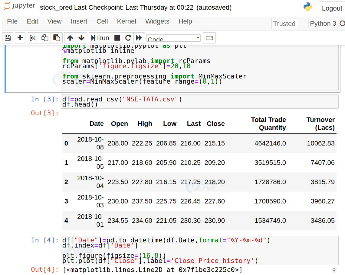
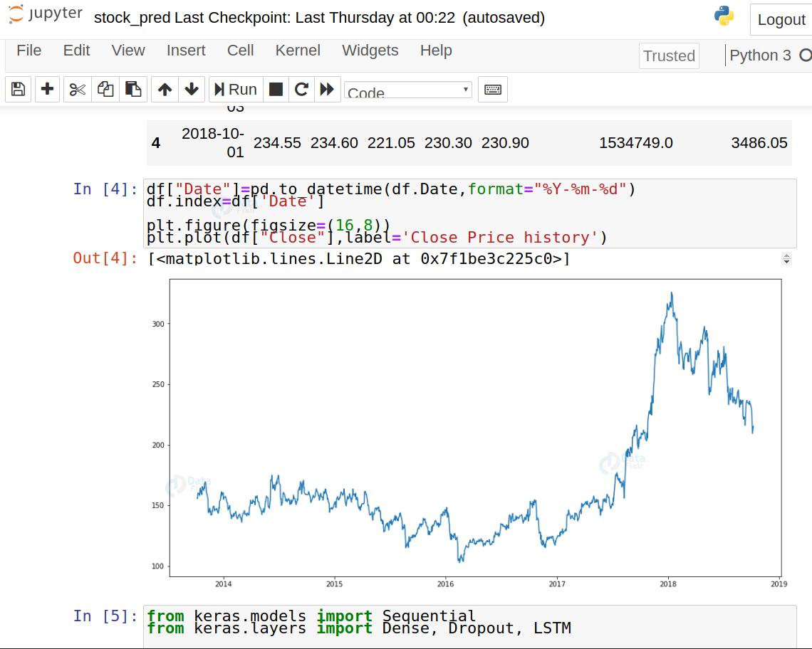
3. Analyze the closing prices from dataframe:
df["Date"]=pd.to_datetime(df.Date,format="%Y-%m-%d")
df.index=df['Date']

plt.figure(figsize=(16,8))
plt.plot(df["Close"],label='Close Price history')
4. Sort the dataset on date time and filter “Date” and “Close” columns:
data=df.sort_index(ascending=True,axis=0)
new_dataset=pd.DataFrame(index=range(0,len(df)),columns=['Date','Close'])

for i in range(0,len(data)):
    new_dataset["Date"][i]=data['Date'][i]
    new_dataset["Close"][i]=data["Close"][i]
5. Normalize the new filtered dataset:
scaler=MinMaxScaler(feature_range=(0,1))
final_dataset=new_dataset.values

train_data=final_dataset[0:987,:]
valid_data=final_dataset[987:,:]

new_dataset.index=new_dataset.Date
new_dataset.drop("Date",axis=1,inplace=True)
scaler=MinMaxScaler(feature_range=(0,1))
scaled_data=scaler.fit_transform(final_dataset)

x_train_data,y_train_data=[],[]

for i in range(60,len(train_data)):
    x_train_data.append(scaled_data[i-60:i,0])
    y_train_data.append(scaled_data[i,0])

x_train_data,y_train_data=np.array(x_train_data),np.array(y_train_data)

x_train_data=np.reshape(x_train_data,(x_train_data.shape[0],x_train_data.shape[1],1))
6. Build and train the LSTM model:
lstm_model=Sequential()
lstm_model.add(LSTM(units=50,return_sequences=True,input_shape=(x_train_data.shape[1],1)))
lstm_model.add(LSTM(units=50))
lstm_model.add(Dense(1))

inputs_data=new_dataset[len(new_dataset)-len(valid_data)-60:].values
inputs_data=inputs_data.reshape(-1,1)
inputs_data=scaler.transform(inputs_data)

lstm_model.compile(loss='mean_squared_error',optimizer='adam')
lstm_model.fit(x_train_data,y_train_data,epochs=1,batch_size=1,verbose=2)
7. Take a sample of a dataset to make stock price predictions using the LSTM model:
X_test=[]
for i in range(60,inputs_data.shape[0]):
    X_test.append(inputs_data[i-60:i,0])
X_test=np.array(X_test)

X_test=np.reshape(X_test,(X_test.shape[0],X_test.shape[1],1))
predicted_closing_price=lstm_model.predict(X_test)
predicted_closing_price=scaler.inverse_transform(predicted_closing_price)
8. Save the LSTM model:
lstm_model.save("saved_model.h5")9. Visualize the predicted stock costs with actual stock costs:
train_data=new_dataset[:987]
valid_data=new_dataset[987:]
valid_data['Predictions']=predicted_closing_price
plt.plot(train_data["Close"])
plt.plot(valid_data[['Close',"Predictions"]])
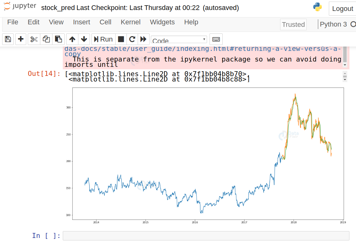
You can observe that LSTM has predicted stocks almost similar to actual stocks.
Build the dashboard using Plotly dash
In this section, we will build a dashboard to analyze stocks. Dash is a python framework that provides an abstraction over flask and react.js to build analytical web applications.
Before moving ahead, you need to install dash. Run the below command in the terminal.
pip3 install dash
pip3 install dash-html-components
pip3 install dash-core-components
Now make a new python file stock_app.py and paste the below script:
import dash
import dash_core_components as dcc
import dash_html_components as html
import pandas as pd
import plotly.graph_objs as go
from dash.dependencies import Input, Output
from keras.models import load_model
from sklearn.preprocessing import MinMaxScaler
import numpy as np
app = dash.Dash()
server = app.server
scaler=MinMaxScaler(feature_range=(0,1))
df_nse = pd.read_csv("./NSE-TATA.csv")
df_nse["Date"]=pd.to_datetime(df_nse.Date,format="%Y-%m-%d")
df_nse.index=df_nse['Date']
data=df_nse.sort_index(ascending=True,axis=0)
new_data=pd.DataFrame(index=range(0,len(df_nse)),columns=['Date','Close'])
for i in range(0,len(data)):
new_data["Date"][i]=data['Date'][i]
new_data["Close"][i]=data["Close"][i]
new_data.index=new_data.Date
new_data.drop("Date",axis=1,inplace=True)
dataset=new_data.values
train=dataset[0:987,:]
valid=dataset[987:,:]
scaler=MinMaxScaler(feature_range=(0,1))
scaled_data=scaler.fit_transform(dataset)
x_train,y_train=[],[]
for i in range(60,len(train)):
x_train.append(scaled_data[i-60:i,0])
y_train.append(scaled_data[i,0])
x_train,y_train=np.array(x_train),np.array(y_train)
x_train=np.reshape(x_train,(x_train.shape[0],x_train.shape[1],1))
model=load_model("saved_model.h5")
inputs=new_data[len(new_data)-len(valid)-60:].values
inputs=inputs.reshape(-1,1)
inputs=scaler.transform(inputs)
X_test=[]
for i in range(60,inputs.shape[0]):
X_test.append(inputs[i-60:i,0])
X_test=np.array(X_test)
X_test=np.reshape(X_test,(X_test.shape[0],X_test.shape[1],1))
closing_price=model.predict(X_test)
closing_price=scaler.inverse_transform(closing_price)
train=new_data[:987]
valid=new_data[987:]
valid['Predictions']=closing_price
df= pd.read_csv("./stock_data.csv")
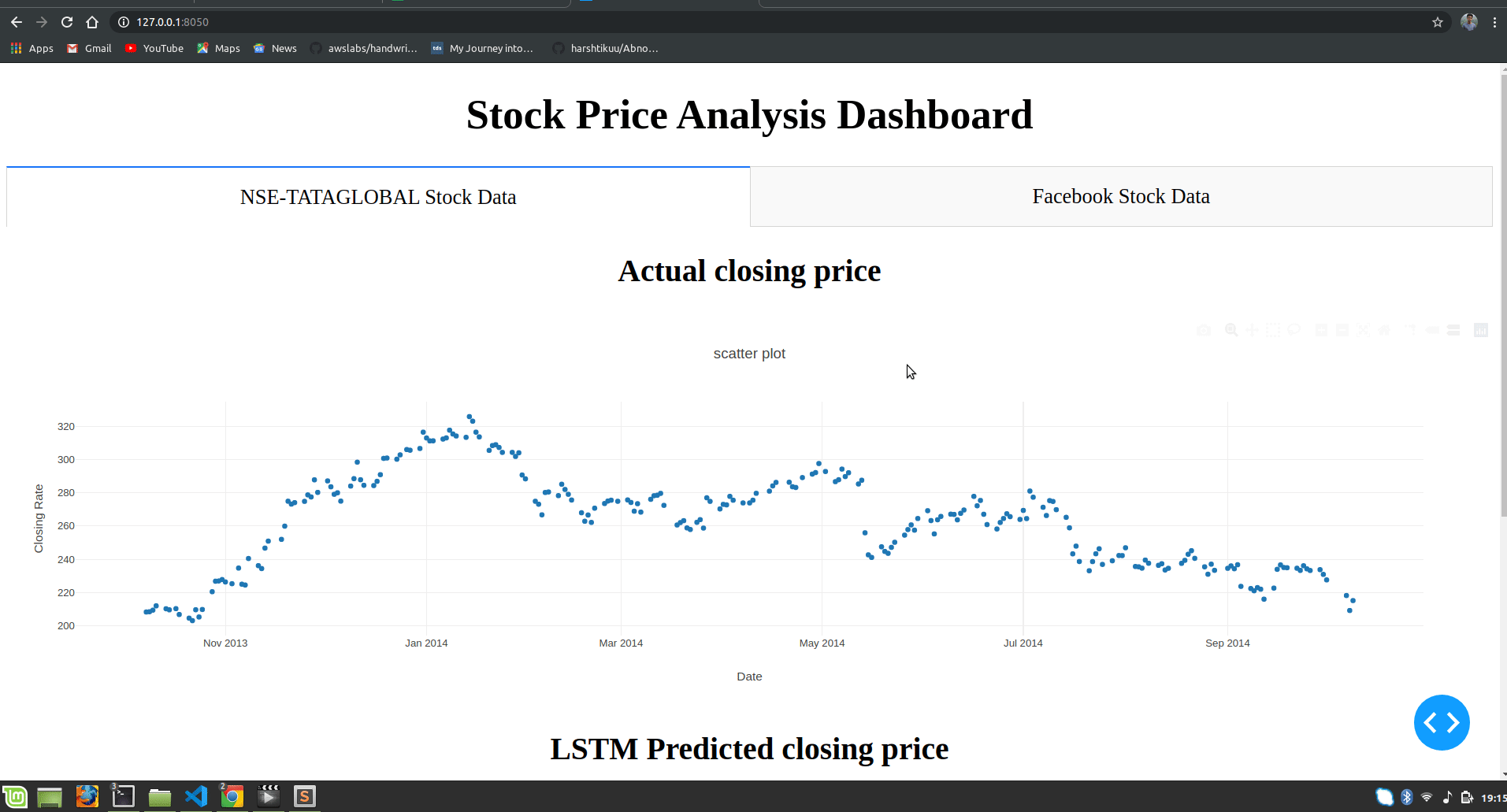
app.layout = html.Div([
html.H1("Stock Price Analysis Dashboard", style={"textAlign": "center"}),
dcc.Tabs(id="tabs", children=[
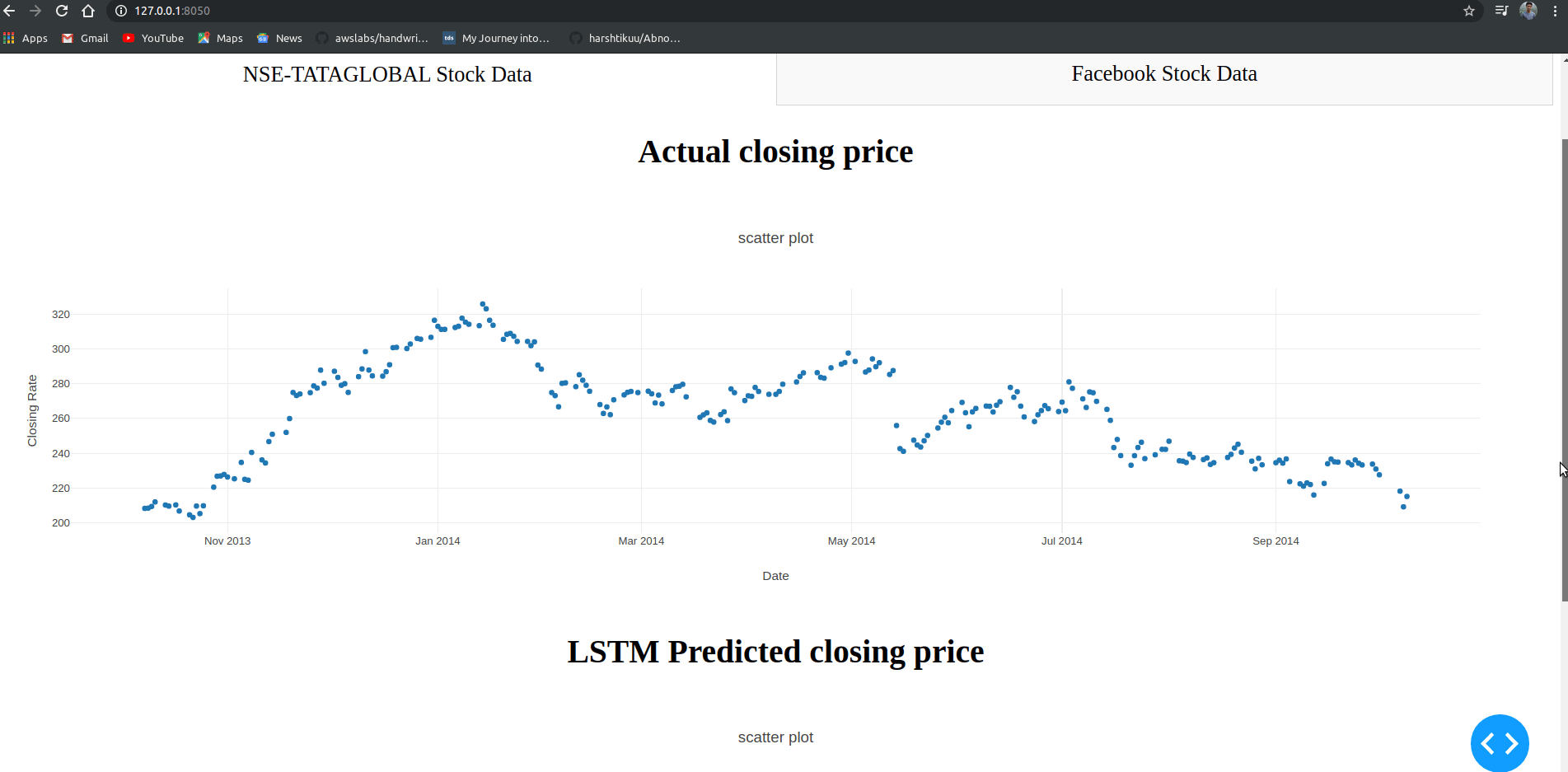
dcc.Tab(label='NSE-TATAGLOBAL Stock Data',children=[
html.Div([
html.H2("Actual closing price",style={"textAlign": "center"}),
dcc.Graph(
id="Actual Data",
figure={
"data":[
go.Scatter(
x=train.index,
y=valid["Close"],
mode='markers'
)
],
"layout":go.Layout(
title='scatter plot',
xaxis={'title':'Date'},
yaxis={'title':'Closing Rate'}
)
}
),
html.H2("LSTM Predicted closing price",style={"textAlign": "center"}),
dcc.Graph(
id="Predicted Data",
figure={
"data":[
go.Scatter(
x=valid.index,
y=valid["Predictions"],
mode='markers'
)
],
"layout":go.Layout(
title='scatter plot',
xaxis={'title':'Date'},
yaxis={'title':'Closing Rate'}
)
}
)
])
]),
dcc.Tab(label='Facebook Stock Data', children=[
html.Div([
html.H1("Facebook Stocks High vs Lows",
style={'textAlign': 'center'}),
dcc.Dropdown(id='my-dropdown',
options=[{'label': 'Tesla', 'value': 'TSLA'},
{'label': 'Apple','value': 'AAPL'},
{'label': 'Facebook', 'value': 'FB'},
{'label': 'Microsoft','value': 'MSFT'}],
multi=True,value=['FB'],
style={"display": "block", "margin-left": "auto",
"margin-right": "auto", "width": "60%"}),
dcc.Graph(id='highlow'),
html.H1("Facebook Market Volume", style={'textAlign': 'center'}),
dcc.Dropdown(id='my-dropdown2',
options=[{'label': 'Tesla', 'value': 'TSLA'},
{'label': 'Apple','value': 'AAPL'},
{'label': 'Facebook', 'value': 'FB'},
{'label': 'Microsoft','value': 'MSFT'}],
multi=True,value=['FB'],
style={"display": "block", "margin-left": "auto",
"margin-right": "auto", "width": "60%"}),
dcc.Graph(id='volume')
], className="container"),
])
])
])
@app.callback(Output('highlow', 'figure'),
[Input('my-dropdown', 'value')])
def update_graph(selected_dropdown):
dropdown = {"TSLA": "Tesla","AAPL": "Apple","FB": "Facebook","MSFT": "Microsoft",}
trace1 = []
trace2 = []
for stock in selected_dropdown:
trace1.append(
go.Scatter(x=df[df["Stock"] == stock]["Date"],
y=df[df["Stock"] == stock]["High"],
mode='lines', opacity=0.7,
name=f'High {dropdown[stock]}',textposition='bottom center'))
trace2.append(
go.Scatter(x=df[df["Stock"] == stock]["Date"],
y=df[df["Stock"] == stock]["Low"],
mode='lines', opacity=0.6,
name=f'Low {dropdown[stock]}',textposition='bottom center'))
traces = [trace1, trace2]
data = [val for sublist in traces for val in sublist]
figure = {'data': data,
'layout': go.Layout(colorway=["#5E0DAC", '#FF4F00', '#375CB1',
'#FF7400', '#FFF400', '#FF0056'],
height=600,
title=f"High and Low Prices for {', '.join(str(dropdown[i]) for i in selected_dropdown)} Over Time",
xaxis={"title":"Date",
'rangeselector': {'buttons': list([{'count': 1, 'label': '1M',
'step': 'month',
'stepmode': 'backward'},
{'count': 6, 'label': '6M',
'step': 'month',
'stepmode': 'backward'},
{'step': 'all'}])},
'rangeslider': {'visible': True}, 'type': 'date'},
yaxis={"title":"Price (USD)"})}
return figure
@app.callback(Output('volume', 'figure'),
[Input('my-dropdown2', 'value')])
def update_graph(selected_dropdown_value):
dropdown = {"TSLA": "Tesla","AAPL": "Apple","FB": "Facebook","MSFT": "Microsoft",}
trace1 = []
for stock in selected_dropdown_value:
trace1.append(
go.Scatter(x=df[df["Stock"] == stock]["Date"],
y=df[df["Stock"] == stock]["Volume"],
mode='lines', opacity=0.7,
name=f'Volume {dropdown[stock]}', textposition='bottom center'))
traces = [trace1]
data = [val for sublist in traces for val in sublist]
figure = {'data': data,
'layout': go.Layout(colorway=["#5E0DAC", '#FF4F00', '#375CB1',
'#FF7400', '#FFF400', '#FF0056'],
height=600,
title=f"Market Volume for {', '.join(str(dropdown[i]) for i in selected_dropdown_value)} Over Time",
xaxis={"title":"Date",
'rangeselector': {'buttons': list([{'count': 1, 'label': '1M',
'step': 'month',
'stepmode': 'backward'},
{'count': 6, 'label': '6M',
'step': 'month',
'stepmode': 'backward'},
{'step': 'all'}])},
'rangeslider': {'visible': True}, 'type': 'date'},
yaxis={"title":"Transactions Volume"})}
return figure
if __name__=='__main__':
app.run_server(debug=True)
Now run this file and open the app in the browser:
python3 stock_app.py
Summary
Stock price prediction helps investors make smart decisions. In this project, we use Python and machine learning to predict the future price of a company’s stock. We use past stock data to train a regression model. It’s a great mix of data analysis, finance, and ML.
Stock price prediction is a machine learning project for beginners; in this tutorial we learned how to develop a stock cost prediction model and how to build an interactive dashboard for stock analysis. We implemented stock market prediction using the LSTM model. OTOH, Plotly dash python framework for building dashboards.
This project is ideal for those interested in finance and ML. It teaches time series forecasting, data visualization, model training, and evaluation. You can build a simple web app or dashboard to show predictions in real-time.
You give me 15 seconds I promise you best tutorials
Please share your happy experience on Google


UnicodeDecodeError: ‘utf-8’ codec can’t decode byte 0xa1 in position 13: invalid start byte,the secind one,i don’t konw why