Sentiment Analysis in Python using Machine Learning

Sentiment analysis or opinion mining is a simple task of understanding the emotions of the writer of a particular text. What was the intent of the writer when writing a certain thing?

We use various natural language processing (NLP) and text analysis tools to figure out what could be subjective information. We need to identify, extract and quantify such details from the text for easier classification and working with the data.

But why do we need sentiment analysis?

Sentiment analysis serves as a fundamental aspect of dealing with customers on online portals and websites for the companies. They do this all the time to classify a comment as a query, complaint, suggestion, opinion, or just love for a product. This way they can easily sort through the comments or questions and prioritize what they need to handle first and even order them in a way that looks better. Companies sometimes even try to delete content that has a negative sentiment attached to it.

It is an easy way to understand and analyze public reception and perception of different ideas and concepts, or a newly launched product, maybe an event or a government policy.

Emotion understanding and sentiment analysis play a huge role in collaborative filtering based recommendation systems. Grouping together people who have similar reactions to a certain product and showing them related products. Like recommending movies to people by grouping them with others that have similar perceptions for a certain show or movie.

Lastly, they are also used for spam filtering and removing unwanted content.

How does sentiment analysis work?

NLP or natural language processing is the basic concept on which sentiment analysis is built upon. Natural language processing is a superclass of sentiment analysis that deals with understanding all kinds of things from a piece of text.

NLP is the branch of AI dealing with texts, giving machines the ability to understand and derive from the text. For tasks such as virtual assistant, query solving, creating and maintaining human-like conversations, summarizing texts, spam detection, sentiment analysis, etc. it includes everything from counting the number of words to a machine writing a story, indistinguishable from human texts.

Sentiment analysis can be classified into various categories based on various criteria. Depending upon the scope it can be classified into document-level sentiment analysis, sentence level sentiment analysis, and sub sentence level or phrase level sentiment analysis.

Also, a very common classification is based on what needs to be done with the data or the reason for sentiment analysis. Examples of which are

• Simple classification of text into positive, negative or neutral. It may also advance into fine grained answers like very positive or moderately positive.
• Aspect-based sentiment analysis- where we figure out the sentiment along with a specific aspect it is related to. Like identifying sentiments regarding various aspects or parts of a car in user reviews, identifying what feature or aspect was appreciated or disliked.
• The sentiment along with an action associated with it. Like mails written to customer support. Understanding if it is a query or complaint or suggestion etc

Based on what needs to be done and what kind of data we need to work with there are two major methods of tackling this problem.

• Matching rules based sentiment analysis: There is a predefined list of words for each type of sentiment needed and then the text or document is matched with the lists. The algorithm then determines which type of words or which sentiment is more prevalent in it.
  This type of rule based sentiment analysis is easy to implement, but lacks flexibility and does not account for context.
• Automatic sentiment analysis: They are mostly based on supervised machine learning algorithms and are actually very useful in understanding complicated texts. Algorithms in this category include support vector machine, linear regression, rnn, and its types. This is what we are gonna explore and learn more about.

In this machine learning project, we will use recurrent neural network for sentiment analysis in python.

Understanding the sentiment analysis system

Recurrent neural networks or RNNs are the go-to method for sequential data. Recurrent neural networks have a memory of their own and remember the input that was given to each node. In a normal feed forward neural network data or information given in the form of input moves forward and never moves backward in any nodes, from the input layer to the hidden layer and out from the output layer. Because these kinds of networks have no memory they do not remember the last input or predict the next input.

When giving out an output an rnn considers what input it is given and also the input that it had received previously, because the information moves in a cycle in an rnn.

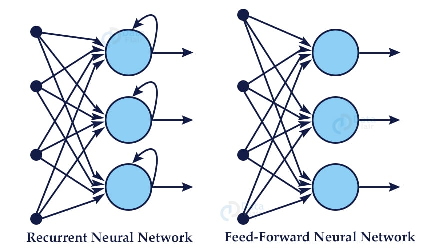
What a recurrent neural network does is creates a copy of the output and loops it back through the network. For example when a sentence is passed through a feedforward network and it takes it word by word, till it reaches the last word. It has no memory of what was fed to it before that. But rnns know the previous inputs as well and can thus also predict what can come next. They are widely used in sequential data.

Recurrent neural networks are not new, were first introduced in the 1980s, but have become a lot popular with the growth of deep learning and its use in sequential data. Still, rnn have their own set of problems, one of the major ones being the vanishing gradient problem. The answer to that being the lstm model.

LSTM or long short term memory models are used to solve these problems. Lstms are a special kind of rnn model that has the capability of learning long term dependencies. They are made to remember long term data. What makes lstm models special is the addition of a memory cell, which is an extra recurrent state and each cell has multiple gates that control the flow of information in and out of the memory cell.

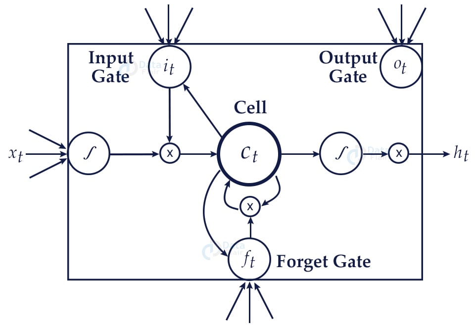
There are three types of gates in an lstm: an input gate, an output gate and a forget gate. The input gate is used to update the cell status, the forget state decides which information is to be stored and which needs to be discarded. The output gate determines the values for the next hidden gates.

Building Sentiment Analysis System

Now that we have a basic understanding of what we need to build we will try implementing it in an easy way.

We will be building a simple sentiment analysis classifier on top of movie reviews, that will classify if the user review of the movie was positive, negative or neutral. For this sentiment analysis python project, we are going to use the imdb movie review dataset.

What is Sentiment Analysis

Sentiment analysis is the process of finding users’ opinions towards a brand, company, or product. It defines the subject behind the social data, after launching a product we can find whether people are liking the product or not. There are many use-cases for sentiment analysis apart from opinion mining.

Download Sentiment Analysis Python Code

Please download the source code sentiment analysis in Python: Sentiment Analysis Python ML Code

Sentiment Analysis Dataset

The dataset which we will use in sentiment analysis is the International Movie Database(IMDb) reviews for 50,000 reviews of movies from all over the world, its a binary classification dataset categorizing each review in a positive or negative. It has 25000 samples for training and 25000 for testing.

You don’t need to download it separately for this project but you can have a look at it on its official website. Because it is a text dataset it is very lightweight around 80MB.

We are going to code all this up in a jupyter notebook on google colab to make use of the free gpu. If you follow along on your own system everything will be pretty much the same except for mounting the google drive for use as a persistent storage option.

• So we begin by mounting our google drive and navigating to the folder where we wanna work.

import os
from google.colab import drive
drive.mount('/content/drive')
 
os.chdir('/content/drive/My Drive/DataFlair/Sentiment')
!ls

Preparation of data

We are going to use pytorch for this project and luckily it comes preinstalled with some functionalities for helping us speeding up our work

The torch.text library is a great tool for nlp projects. It has a loader for some common nlp datasets like the one we are going to use today, also complete pipeline for abstraction of vectorization of data, data loaders and iteration of data.

import random
import torch
from torchtext.legacy import data
from torchtext.legacy import datasets
 
seed = 42
 
torch.manual_seed(seed)
torch.backends.cudnn.deterministic = True
device = torch.device('cuda' if torch.cuda.is_available() else 'cpu')
 
txt = data.Field(tokenize = 'spacy',
                  tokenizer_language = 'en_core_web_sm',
                  include_lengths = True)
 
labels = data.LabelField(dtype = torch.float)

We are going to use the field method of the data class to decide how data needs to be preprocessed. The parameters we pass in there will determine the preprocessing, we are just going to tweak some parameters and leave the rest to default.

The first parameter, our tokenizer(that determines how the sentences are going to be broken down or tokenized in nlp standard) is spacy, which is a powerful tool for one line tokenization. We recommend using this, but the default is just tokenizing the string based on blank spaces. Also we need to tell the spacy tokenizer which language model to use for the task.

We also set the random seed to a certain number, which could be any but we mention it just for reproducibility purposes. You could change it or even omit it without any significant effect. We also want to use cuda and also the gpu available to us so we use swt that as well.

train_data, test_data = datasets.IMDB.splits(txt, labels)
train_data, valid_data = train_data.split(random_state = random.seed(seed))
num_words = 25_000
 
txt.build_vocab(train_data, 
                 max_size = num_words, 
                 vectors = "glove.6B.100d", 
                 unk_init = torch.Tensor.normal_)
 
labels.build_vocab(train_data)

Here we have downloaded the imdb dataset for python sentiment analysis and divided it into train test and validation split. The dataset is already divided into a train and test set, we further create a validation set from it.

We further limit the number of words the model will learn to 25000, this will choose the most used 25000 words from the dataset and use them for training. Significantly reducing the work of the model without any real loss in accuracy.

btch_size = 64
 
train_itr, valid_itr, test_itr = data.BucketIterator.splits(
    (train_data, valid_data, test_data), 
    batch_size = btch_size,
    sort_within_batch = True,
    device = device)

We are now creating a training, testing and validation batch from the data that we have for preparing it to be fed to the model in the form of batches of 64 samples at a time. Reduce this if you get out of memory error.

Defining python sentiment analysis model

We now prepare the model and define its architecture. We are using a lstm rnn for our task. We will be using a multi layer bidirectional rnn. That means there will be multiple rnn layers stacked on top of each other.

Bidirectional RNNs have an advantage of having more context than a single directional network. For example, in a sentence flowing forward through a model, if a model has to guess the next word, it would do so on the basis of previous knowledge. But in a bidirectional network it will also have the knowledge of what’s next due to two networks flowing in opposite directions stacked on top of each other. The input flows in the opposite direction as well as sequence. A sentence “i love DataFlair” will flow in the first network as “i” , “love” , “DataFlair” but in the second it will flow like “DataFlair” , “love” , “i”. This provides better context and relation in the data to the network.

The hidden state output from the first layer will be the input to the next layer, also each layer has its independent hidden nodes.

We use nn.LSTM layers instead of normal nn.RNN layers

We pass everything through an embedding layer which is just a representation of words in lower-dimensional space. Simply put to place the words such that similar words are grouped together.

import torch.nn as nn
 
class RNN(nn.Module):
    def __init__(self, word_limit, dimension_embedding, dimension_hidden, dimension_output, num_layers, 
                 bidirectional, dropout, pad_idx):
        
        super().__init__()
        
        self.embedding = nn.Embedding(word_limit, dimension_embedding, padding_idx = pad_idx)
        
        self.rnn = nn.LSTM(dimension_embedding, 
                           dimension_hidden, 
                           num_layers=num_layers, 
                           bidirectional=bidirectional, 
                           dropout=dropout)
        
        self.fc = nn.Linear(dimension_hidden * 2, dimension_output)
        
        self.dropout = nn.Dropout(dropout)
        
    def forward(self, text, len_txt):
        
        
        embedded = self.dropout(self.embedding(text))
               
 
        packed_embedded = nn.utils.rnn.pack_padded_sequence(embedded, len_txt.to('cpu'))
        
        packed_output, (hidden, cell) = self.rnn(packed_embedded)
        
        output, output_lengths = nn.utils.rnn.pad_packed_sequence(packed_output)
 
        
        hidden = self.dropout(torch.cat((hidden[-2,:,:], hidden[-1,:,:]), dim = 1))
                            
        return self.fc(hidden)

We define the parameters for python sentiment analysis model and pass it to an instance of the model class we just defined. The number of input parameters, hidden layer, and the output dimension along with throughput rate and bidirectionality boolean is defined. We also pass the pad token index from the vocabulary that we created earlier.

dimension_input = len(txt.vocab)
dimension_embedding = 100
dimension_hddn = 256
dimension_out = 1
layers = 2
bidirectional = True
dropout = 0.5
idx_pad = txt.vocab.stoi[txt.pad_token]
 
model = RNN(dimension_input, 
            dimension_embedding, 
            dimension_hddn, 
            dimension_out, 
            layers, 
            bidirectional, 
            dropout, 
            idx_pad)

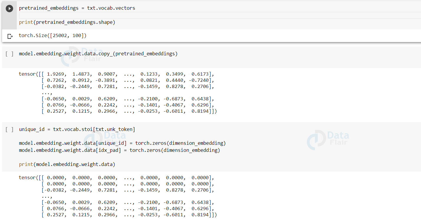
Now we print some details about our model. Getting the number of trainable parameters that are present there in the model.

We then get the pre-trained embedding weights and copy them to our model so that it does not need to learn the embeddings, and can directly focus on the job at hand that is learning the sentiments related to those embeddings.

Pretrained embedding weights are placed in place of the initial ones.

def count_parameters(model):
    return sum(p.numel() for p in model.parameters() if p.requires_grad)
 
print(f'The model has {count_parameters(model):,} trainable parameters')
pretrained_embeddings = txt.vocab.vectors
 
print(pretrained_embeddings.shape)
unique_id = txt.vocab.stoi[txt.unk_token]
 
model.embedding.weight.data[unique_id] = torch.zeros(dimension_embedding)
model.embedding.weight.data[idx_pad] = torch.zeros(dimension_embedding)
 
print(model.embedding.weight.data)

Now we define some parameters regarding the model, that is the optimizer we are going to use and the criterion of loss we need. We chose adam optimizer for fast convergence of the model along with logistic loss function. We place the model and the criterion on the gpu.

import torch.optim as optim
 
optimizer = optim.Adam(model.parameters())
criterion = nn.BCEWithLogitsLoss()
 
model = model.to(device)
criterion = criterion.to(device)

Training of the model

We now begin the necessary functions for training and evaluation of sentiment analysis model.

The first one being the binary accuracy function, which we’ll use for getting the accuracy of the model each time.

def bin_acc(preds, y):
   
    predictions = torch.round(torch.sigmoid(preds))
    correct = (predictions == y).float() 
    acc = correct.sum() / len(correct)
    return acc

We define the function for training and evaluating the models. The process here is standard. We start by looping through the number of epochs and the number of iterations in each epoch is according to the batch size that we defined. We pass the text to the model, get the predictions from it, calculate the loss for each iteration and then backward propagate that loss.

The only major change in the evaluating function from the training function is that we do not backward propagate the loss through the model and use torch.nograd basically signifying no gradient descent while evaluating.

def train(model, itr, optimizer, criterion):
    
    epoch_loss = 0
    epoch_acc = 0
    
    model.train()
    
    for i in itr:
        
        optimizer.zero_grad()
        
        text, len_txt = i.text
        
        predictions = model(text, len_txt).squeeze(1)
        
        loss = criterion(predictions, i.label)
        
        acc = bin_acc(predictions, i.label)
        
        loss.backward()
        
        optimizer.step()
        
        epoch_loss += loss.item()
        epoch_acc += acc.item()
        
    return epoch_loss / len(itr), epoch_acc / len(itr)
 
def evaluate(model, itr, criterion):
    
    epoch_loss = 0
    epoch_acc = 0
    
    model.eval()
    
    with torch.no_grad():
    
        for i in itr:
 
            text, len_txt = i.text
            
            predictions = model(text, len_txt).squeeze(1)
            
            loss = criterion(predictions, i.label)
            
            acc = bin_acc(predictions, i.label)
 
            epoch_loss += loss.item()
            epoch_acc += acc.item()
        
    return epoch_loss / len(itr), epoch_acc / len(itr)

We build a helper function epoch_time for calculating the time each epoch takes to complete its run and print it. We set the number of epochs to 5 and then begin our training. Adding the training and validation loss at each stage, if we need to understand or plot the training curve at a later point. We save the python sentiment analysis model that has the best validation loss.

import time
 
def epoch_time(start_time, end_time):
    used_time = end_time - start_time
    used_mins = int(used_time / 60)
    used_secs = int(used_time - (used_mins * 60))
    return used_mins, used_secs
num_epochs = 5
 
best_valid_loss = float('inf')
 
for epoch in range(num_epochs):
 
    start_time = time.time()
    
    train_loss, train_acc = train(model, train_itr, optimizer, criterion)
    valid_loss, valid_acc = evaluate(model, valid_itr, criterion)
    
    end_time = time.time()
 
    epoch_mins, epoch_secs = epoch_time(start_time, end_time)
    
    if valid_loss < best_valid_loss:
        best_valid_loss = valid_loss
        torch.save(model.state_dict(), 'tut2-model.pt')
    
    print(f'Epoch: {epoch+1:02} | Epoch Time: {epoch_mins}m {epoch_secs}s')
    print(f'\tTrain Loss: {train_loss:.3f} | Train Acc: {train_acc*100:.2f}%')
    print(f'\t Val. Loss: {valid_loss:.3f} |  Val. Acc: {valid_acc*100:.2f}%')


100%|█████████▉| 398630/400000 [00:30<00:00, 25442.01it/s]Epoch: 01 | Epoch Time: 0m 37s
  Train Loss: 0.658 | Train Acc: 60.15%
   Val. Loss: 0.675 |  Val. Acc: 60.89%
Epoch: 02 | Epoch Time: 0m 38s
  Train Loss: 0.653 | Train Acc: 60.98%
   Val. Loss: 0.606 |  Val. Acc: 68.85%
Epoch: 03 | Epoch Time: 0m 40s
  Train Loss: 0.490 | Train Acc: 77.06%
   Val. Loss: 0.450 |  Val. Acc: 80.64%
Epoch: 04 | Epoch Time: 0m 40s
  Train Loss: 0.390 | Train Acc: 83.21%
   Val. Loss: 0.329 |  Val. Acc: 86.56%
Epoch: 05 | Epoch Time: 0m 40s
  Train Loss: 0.321 | Train Acc: 86.95%
   Val. Loss: 0.432 |  Val. Acc: 81.71%

Testing sentiment analysis model

We load the saved checkpoint of the model and test it on the test set that we created earlier. During the dry run of python sentiment analysis model, we achieved a decent accuracy score of 85.83%.

model.load_state_dict(torch.load('tut2-model.pt'))
 
test_loss, test_acc = evaluate(model, test_itr, criterion)
 
print(f'Test Loss: {test_loss:.3f} | Test Acc: {test_acc*100:.2f}%')

We can also check the model on our data. This is trained to classify the movie reviews into positive, negative, and neutral, therefore we will pass to it relatable data for checking. So for that we will import and load spacy for tokenizing the data we need to give to the model. In the beginning, while defining the preprocessing we used spacy built-in torch.text, but here we are not using batches, and the preprocessing that we need to do can be handled by the spacy library. We define a predict sentiment function for this. After the preprocessing, we convert it into tensors and ready to be passed to the model

import spacy
nlp = spacy.load('en_core_web_sm')
 
def pred(model, sentence):
    model.eval()
    tokenized = [tok.text for tok in nlp.tokenizer(sentence)]
    indexed = [txt.vocab.stoi[t] for t in tokenized]
    length = [len(indexed)]
    tensor = torch.LongTensor(indexed).to(device)
    tensor = tensor.unsqueeze(1)
    length_tensor = torch.LongTensor(length)
    prediction = torch.sigmoid(model(tensor, length_tensor))
    return prediction.item()

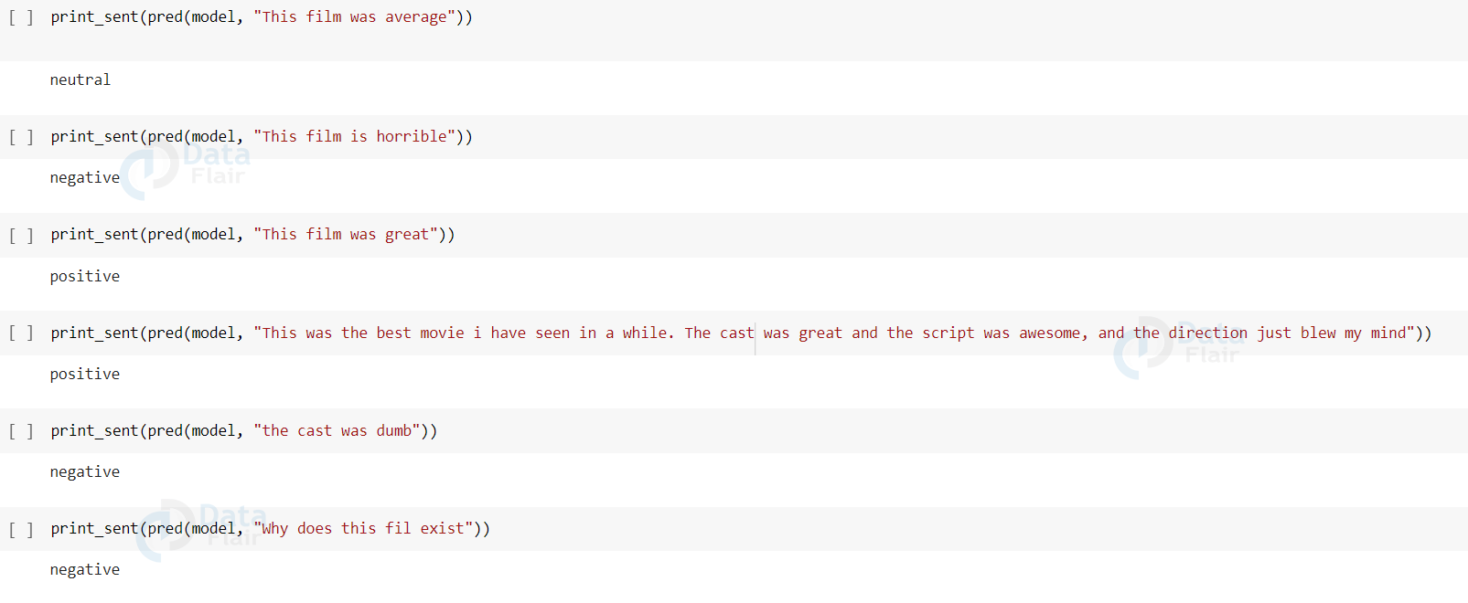
We define another helper function that will print the sentiment of the comment based on the score that the model provides.

sent=["positive","neutral","negative"]
def print_sent(x):
  if (x<0.3): print(sent[0])
  elif (x>0.3 and x<0.7): print(sent[1])
  else: print(sent[2])

Now we just pass any data and test what does the model think about it

print_sent(pred(model, "This film was great"))
positive

Python Sentiment Analysis Output

Summary

We have successfully developed python sentiment analysis model based on lstm techniques that is pretty robust and highly accurate. As discussed earlier, sentiment analysis has many use-cases based on requirements we can use it. We can similarly train it on any other kind of data just by changing the dataset according to our needs. We can use this sentiment analysis model in all different ways possible.