Credit Card Fraud Detection with Python & Machine Learning

For any bank or financial organization, credit card fraud detection is of utmost importance. We have to spot potential fraud so that consumers can not bill for goods that they haven’t purchased. The aim is, therefore, to create a classifier that indicates whether a requested transaction is a fraud.

About Credit Card Fraud Detection

In this machine learning project, we solve the problem of detecting credit card fraud transactions using machine numpy, scikit learn, and few other python libraries. We overcome the problem by creating a binary classifier and experimenting with various machine learning techniques to see which fits better.

Credit Card Fraud Dataset

The dataset consists of 31 parameters. Due to confidentiality issues, 28 of the features are the result of the PCA transformation. “Time’ and “Amount” are the only aspects that were not modified with PCA.

There are a total of 284,807 transactions with only 492 of them being fraud. So, the label distribution suffers from imbalance issues.

Please download the dataset for credit card fraud detection project: Anonymized Credit Card Transactions for Fraud Detection

Tools and Libraries used

We use the following libraries and frameworks in credit card fraud detection project.

• Python – 3.x
• Numpy – 1.19.2
• Scikit-learn – 0.24.1
• Matplotlib – 3.3.4
• Imblearn – 0.8.0
• Collections, Itertools

Credit Card Fraud Project Code

Please download the source code of the credit card fraud detection project (which is explained below): Credit Card Fraud Detection Machine Learning Code

Steps to Develop Credit Card Fraud Classifier in Machine Learning

Our approach to building the classifier is discussed in the steps:

1. Perform Exploratory Data Analysis (EDA) on our dataset
2. Apply different Machine Learning algorithms to our dataset
3. Train and Evaluate our models on the dataset and pick the best one.

Step 1. Perform Exploratory Data Analysis (EDA)

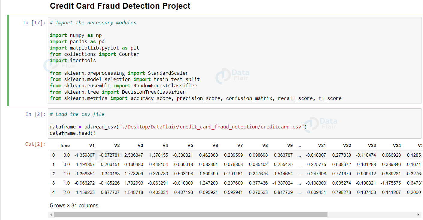
There are a total of 284,807 transactions with only 492 of them being fraud. Let’s import the necessary modules, load our dataset, and perform EDA on our dataset. Here is a peek at our dataset:

import pandas as pd
from collections import Counter
import itertools

# Load the csv file

dataframe = pd.read_csv("./Desktop/DataFlair/credit_card_fraud_detection/creditcard.csv")
dataframe.head()

Output:

Now, check for null values in the credit card dataset. Luckily, there aren’t any null or NaN values in our dataset.

dataframe.isnull().values.any()

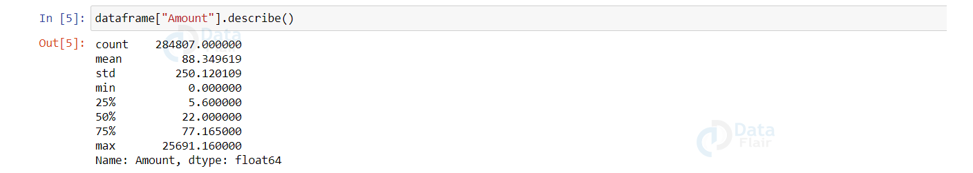
The feature we are most interested in is the “Amount”. Here is the summary of the feature.

dataframe["Amount"].describe()

Output:

Now, let’s check the number of occurrences of each class label and plot the information using matplotlib.

non_fraud = len(dataframe[dataframe.Class == 0])
fraud = len(dataframe[dataframe.Class == 1])
fraud_percent = (fraud / (fraud + non_fraud)) * 100

print("Number of Genuine transactions: ", non_fraud)
print("Number of Fraud transactions: ", fraud)
print("Percentage of Fraud transactions: {:.4f}".format(fraud_percent))

Let’s plot the above information using matplotlib.

import matplotlib.pyplot as plt

labels = ["Genuine", "Fraud"]
count_classes = dataframe.value_counts(dataframe['Class'], sort= True)
count_classes.plot(kind = "bar", rot = 0)
plt.title("Visualization of Labels")
plt.ylabel("Count")
plt.xticks(range(2), labels)
plt.show()

Output:

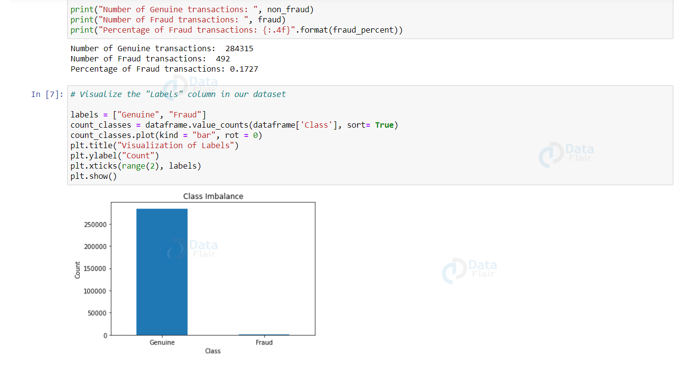
We can observe that the genuine transactions are over 99%! This is not good.

Let’s apply scaling techniques on the “Amount” feature to transform the range of values. We drop the original “Amount” column and add a new column with the scaled values. We also drop the “Time” column as it is irrelevant.

import numpy as np
from sklearn.preprocessing import StandardScaler

scaler = StandardScaler()
dataframe["NormalizedAmount"] = scaler.fit_transform(dataframe["Amount"].values.reshape(-1, 1))
dataframe.drop(["Amount", "Time"], inplace= True, axis= 1)

Y = dataframe["Class"]
X = dataframe.drop(["Class"], axis= 1)

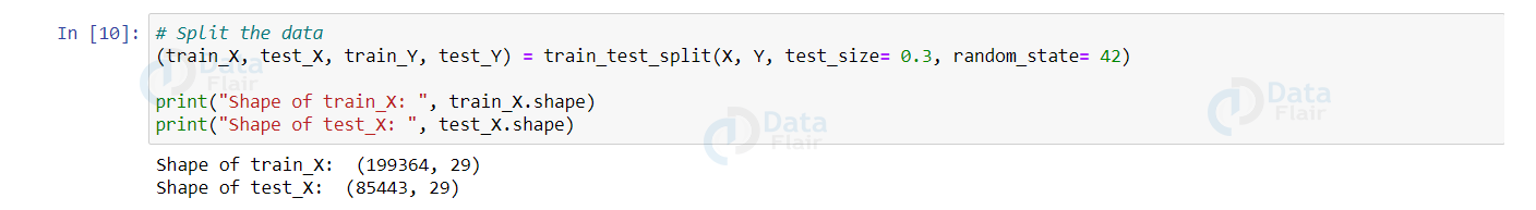
Now, it’s time to split credit card data with a split of 70-30 using train_test_split().

from sklearn.model_selection import train_test_split

(train_X, test_X, train_Y, test_Y) = train_test_split(X, Y, test_size= 0.3, random_state= 42)

print("Shape of train_X: ", train_X.shape)
print("Shape of test_X: ", test_X.shape)

Output:

Step 2: Apply Machine Learning Algorithms to Credit Card Dataset

Let’s train different models on our dataset and observe which algorithm works better for our problem. This is actually a binary classification problem as we have to predict only 1 of the 2 class labels. We can apply a variety of algorithms for this problem like Random Forest, Decision Tree, Support Vector Machine algorithms, etc.

In this machine learning project, we build Random Forest and Decision Tree classifiers and see which one works best. We address the “class imbalance” problem by picking the best-performed model.

But before we go into the code, let’s understand what random forests and decision trees are.

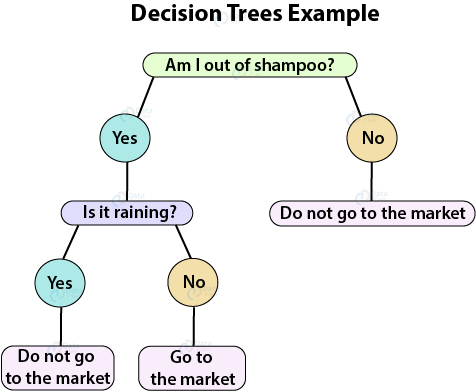
The Decision Tree algorithm is a supervised machine learning algorithm used for classification and regression tasks. The algorithm’s aim is to build a training model that predicts the value of a target class variable by learning simple if-then-else decision rules inferred from the training data.

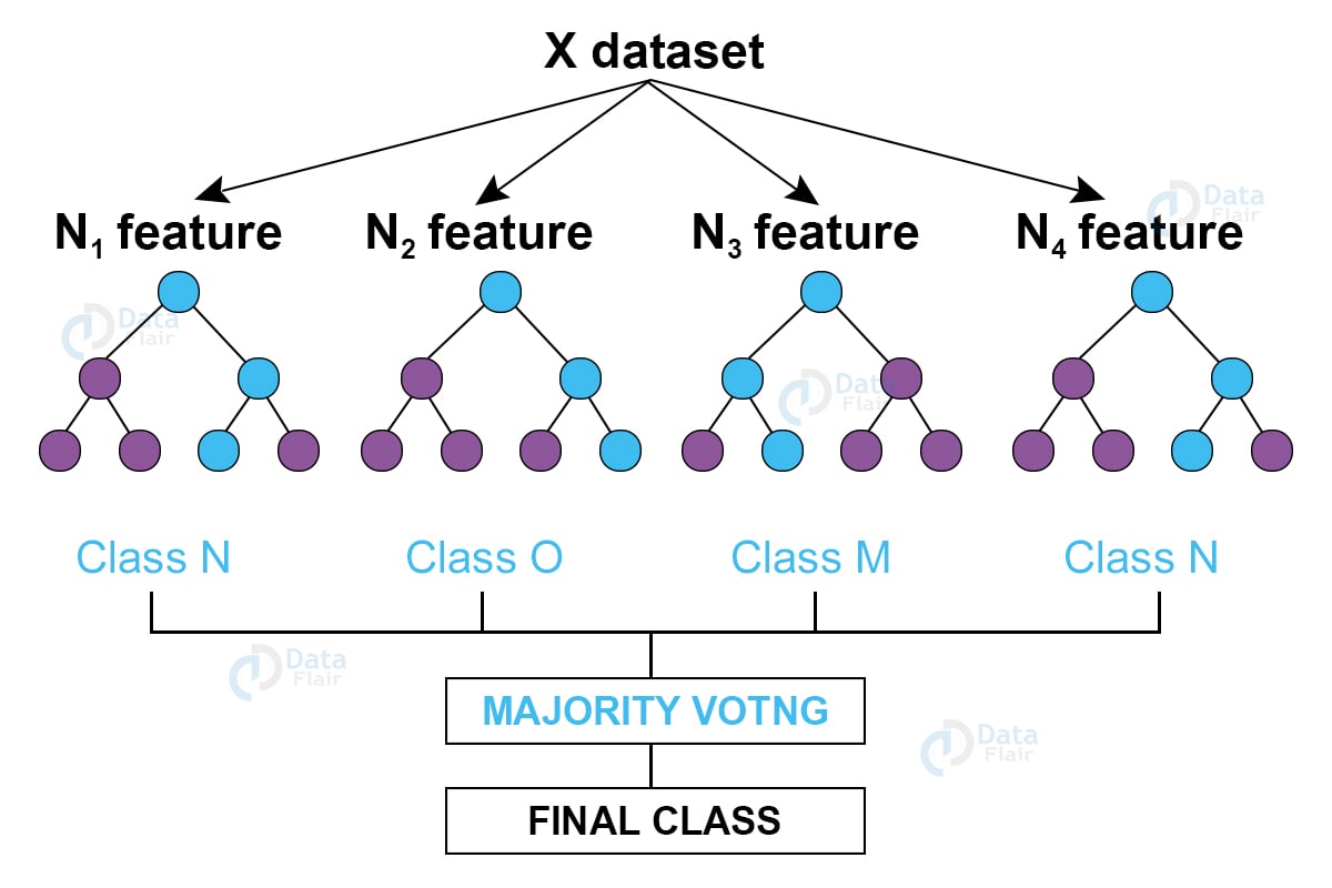
Random forest (one of the most popular algorithms) is a supervised machine learning algorithm. It creates a “forest” out of an ensemble of “decision trees”, which are normally trained using the “bagging” technique. The bagging method’s basic principle is that combining different learning models improves the outcome.

To get a more precise and reliable forecast, random forest creates several decision trees and merges them.

Let’s build the Random Forest and Decision Tree Classifiers. They are present in the sklearn package in the form of RandomForestClassifier() and DecisionTreeClassifier() respectively.

from sklearn.ensemble import RandomForestClassifier
from sklearn.tree import DecisionTreeClassifier

#Decision Tree
decision_tree = DecisionTreeClassifier()

# Random Forest
random_forest = RandomForestClassifier(n_estimators= 100)

Step 3: Train and Evaluate our Models on the Dataset

Now, Let’s train and evaluate the newly created models on the dataset and pick the best one.

Train the decision tree and random forest models on the dataset using the fit() function. Record the predictions made by the models using the predict() function and evaluate.

Let’s visualize the scores of each of our credit card fraud classifiers.

decision_tree.fit(train_X, train_Y)
predictions_dt = decision_tree.predict(test_X)
decision_tree_score = decision_tree.score(test_X, test_Y) * 100

random_forest.fit(train_X, train_Y)
predictions_rf = random_forest.predict(test_X)
random_forest_score = random_forest.score(test_X, test_Y) * 100

print("Random Forest Score: ", random_forest_score)
print("Decision Tree Score: ", decision_tree_score)

Output:

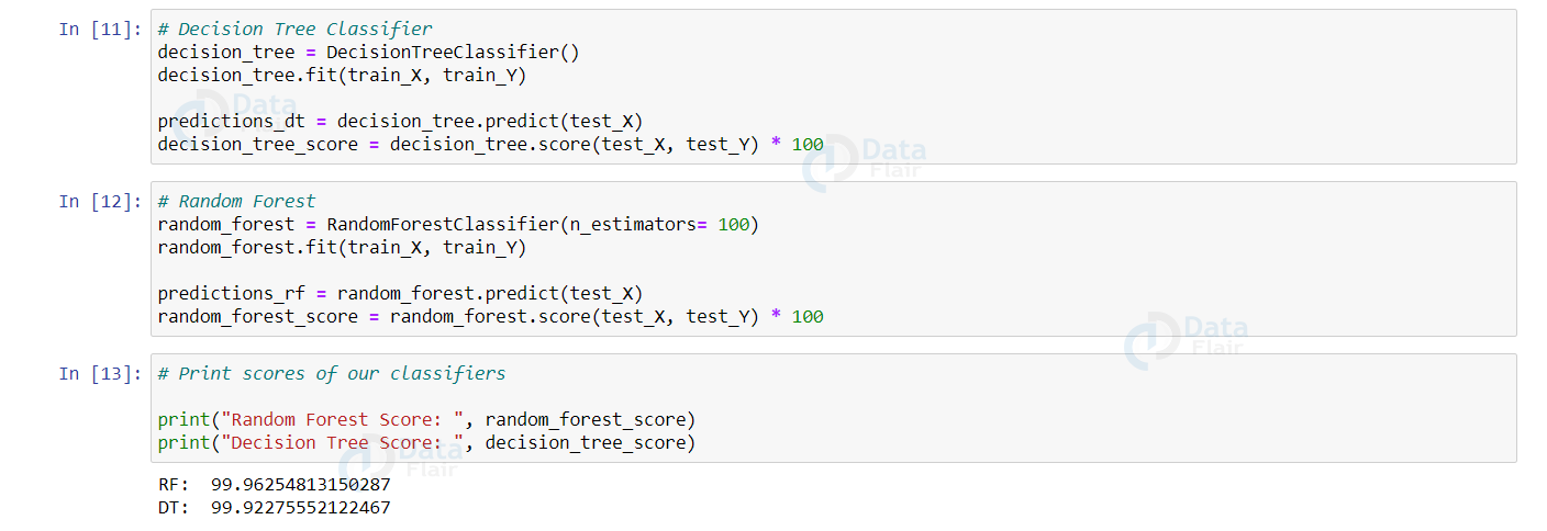
The Random Forest classifier has slightly an edge over the Decision Tree classifier.

Let’s create a function to print the metrics: accuracy, precision, recall, and f1-score.

from sklearn.metrics import accuracy_score, precision_score, confusion_matrix, recall_score, f1_score


def metrics(actuals, predictions):
    print("Accuracy: {:.5f}".format(accuracy_score(actuals, predictions)))
    print("Precision: {:.5f}".format(precision_score(actuals, predictions)))
    print("Recall: {:.5f}".format(recall_score(actuals, predictions)))
    print("F1-score: {:.5f}".format(f1_score(actuals, predictions)))

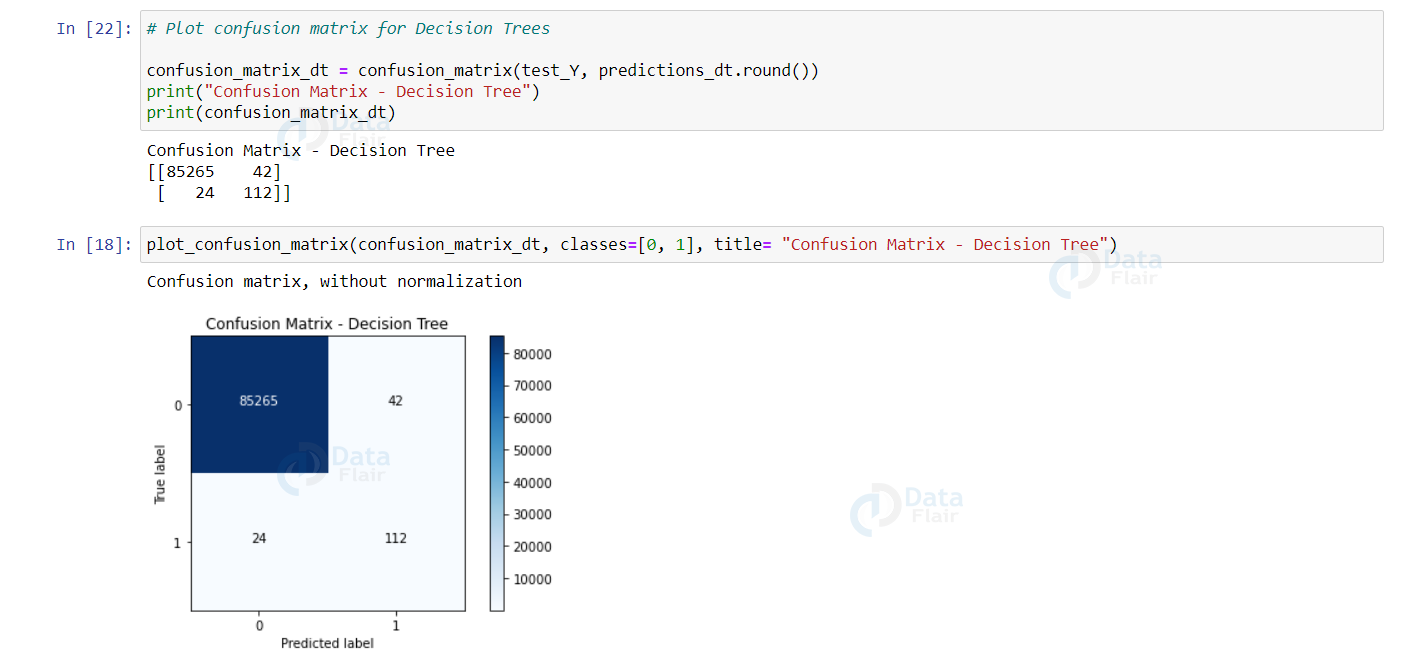
Let’s visualize the confusion matrix and the evaluation metrics of our Decision Tree model.

confusion_matrix_dt = confusion_matrix(test_Y, predictions_dt.round())
print("Confusion Matrix - Decision Tree")
print(confusion_matrix_dt)
plot_confusion_matrix(confusion_matrix_dt, classes=[0, 1], title= "Confusion Matrix - Decision Tree")

Output:

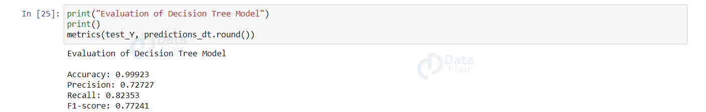
print("Evaluation of Decision Tree Model")
print()
metrics(test_Y, predictions_dt.round())

Output:

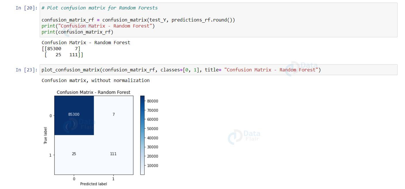
Let’s visualize the confusion matrix and the evaluation metrics of our Random Forest model.

confusion_matrix_rf = confusion_matrix(test_Y, predictions_rf.round())
print("Confusion Matrix - Random Forest")
print(confusion_matrix_rf)
plot_confusion_matrix(confusion_matrix_rf, classes=[0, 1], title= "Confusion Matrix - Random Forest")

Output:

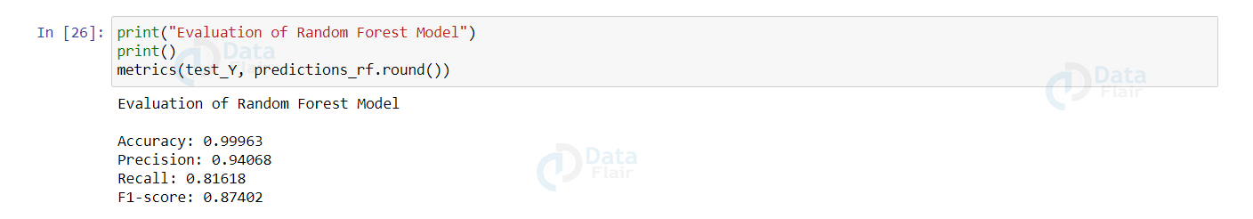
print("Evaluation of Random Forest Model")
print()
metrics(test_Y, predictions_rf.round())

Output:

Address the Class-Imbalance issue

The Random Forest model works better than Decision Trees. But, if we observe our dataset suffers a serious problem of class imbalance. The genuine (not fraud) transactions are more than 99% with the credit card fraud transactions constituting 0.17%.

With such a distribution, if we train our model without taking care of the imbalance issues, it predicts the label with higher importance given to genuine transactions (as there is more data about them) and hence obtains more accuracy.

The class imbalance problem can be solved by various techniques. Oversampling is one of them.

Oversample the minority class is one of the approaches to address the imbalanced datasets. The easiest solution entails doubling examples in the minority class, even though these examples contribute no new data to the model.

Instead, new examples may be generated by replicating existing ones. The Synthetic Minority Oversampling Technique, or SMOTE for short, is a method of data augmentation for the minority class.

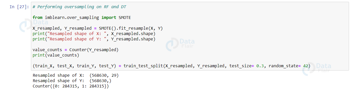
The above SMOTE is present in the imblearn package. Let’s import that and resample our data.

In the following code below, we resampled our data and we split it using train_test_split() with a split of 70-30.

from imblearn.over_sampling import SMOTE

X_resampled, Y_resampled = SMOTE().fit_resample(X, Y)
print("Resampled shape of X: ", X_resampled.shape)
print("Resampled shape of Y: ", Y_resampled.shape)

value_counts = Counter(Y_resampled)
print(value_counts)

(train_X, test_X, train_Y, test_Y) = train_test_split(X_resampled, Y_resampled, test_size= 0.3, random_state= 42)

Output:

As the Random Forest algorithm performed better than the Decision Tree algorithm, we will apply the Random Forest algorithm to our resampled data.

rf_resampled = RandomForestClassifier(n_estimators = 100)
rf_resampled.fit(train_X, train_Y)

predictions_resampled = rf_resampled.predict(test_X)
random_forest_score_resampled = rf_resampled.score(test_X, test_Y) * 100

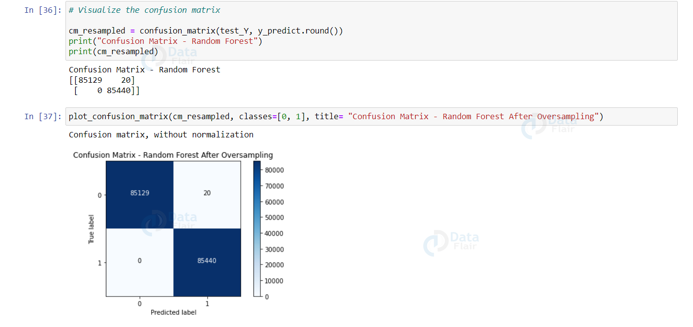
Let’s visualize the predictions of our model and plot the confusion matrix.

cm_resampled = confusion_matrix(test_Y, y_predict.round())
print("Confusion Matrix - Random Forest")
print(cm_resampled)
plot_confusion_matrix(cm_resampled, classes=[0, 1], title= "Confusion Matrix - Random Forest After Oversampling")

Output:

print("Evaluation of Random Forest Model")
print()

metrics(test_Y, predictions_resampled.round())

Output:

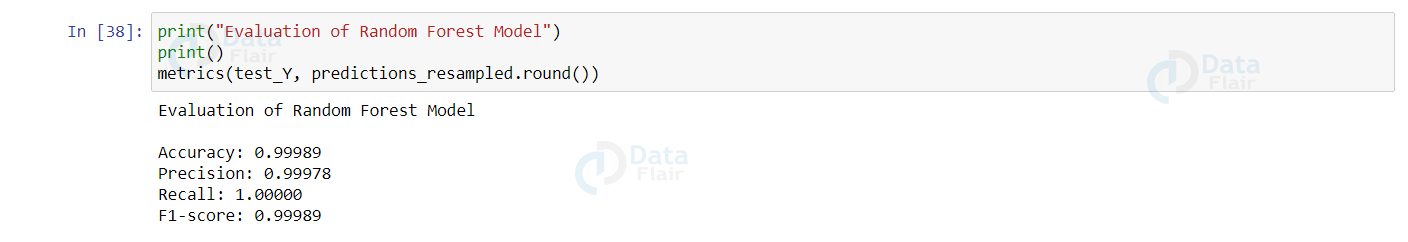
Now, it is clearly evident that our model performed much better than our previous Random Forest classifier without oversampling.

Summary

In this python machine learning project, we built a binary classifier using the Random Forest algorithm to detect credit card fraud transactions. Through this project, we understood and applied techniques to address the class imbalance issues and achieved an accuracy of more than 99%.