Brain Tumor Classification using Machine Learning

Deep learning (subfield of machine learning) has gained prominence in almost every field where decision-making is involved in recent years, spanning economics, health care, marketing, and sales. In the field of healthcare, machine learning & deep learning have shown promising results in a variety of fields, namely disease diagnosis with medical imaging, surgical robots, and boosting hospital performance.

One such application of deep learning to detect brain tumors from MRI scan images.

About Brain Tumor Classification Project

In this machine learning project, we build a classifier to detect the brain tumor (if any) from the MRI scan images. By now it is evident that this is a binary classification problem. Examples of such binary classification problems are Spam or Not spam, Credit card fraud (Fraud or Not fraud).

Brain Tumor Classification Dataset

Please download the dataset for brain tumor classification: Brain Tumor Dataset

The images are split into two folders yes and no each containing images with and without brain tumors respectively. There are a total of 253 images.

Tools and Libraries used

Brain tumor detection project uses the below libraries and frameworks:

• Python – 3.x
• TensorFlow – 2.4.1
• Keras – 2.4.0
• Numpy – 1.19.2
• Scikit-learn – 0.24.1
• Matplotlib – 3.3.4
• OpenCV – 4.5.2

Brain Tumor Project Code

Please download the source code of the brain tumor detection project (which is explained below): Brain Tumor Classification Machine Learning Code

Steps to Develop Brain Tumor Classifier in Machine Learning

Our approach to building the classifier is discussed in the steps:

1. Perform Exploratory Data Analysis (EDA) on brain tumor dataset
2. Build a CNN model
3. Train and Evaluate our model on the dataset

Step 1. Perform Exploratory Data Analysis (EDA)

The brain tumor dataset contains 2 folders “no” and “yes” with 98 and 155 images each. Load the folders containing the images to our current working directory. Using the imutils module, we extract the paths for all the images and store them in a list called image_paths.

from imutils import paths
import matplotlib.pyplot as plt
import argparse
import os
import cv2

# Load the images directories
path = "./Desktop/DataFlair/brain_tumor_dataset"
image_paths = list(paths.list_images(path))

Now, we iterate over each of the paths and extract the directory name (no or yes in our case which acts as the label), and resize the image size to 224×224 pixels. The imread() function of the cv2 module converts brain tumor images to pixel information.

images = []
labels = []

for image_path in image_paths:
    label = image_path.split(os.path.sep)[-2]
    image = cv2.imread(image_path)
    image = cv2.resize(image, (224, 224))

    images.append(image)
    labels.append(label)

Let’s plot an image using the matplotlib module.

def plot_image(image):
    plt.imshow(image)

plot_image(images[0])

Output:

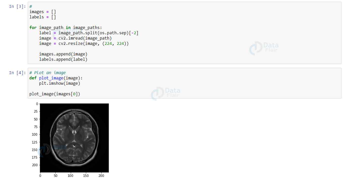
As you can see, we have stored the image and its respective label in lists. But the labels are strings which can’t be interpreted by machines. So, apply One-hot encoding to the labels.

Also, normalize the images and convert our lists to numpy arrays to further split our dataset.

from sklearn.preprocessing import LabelBinarizer
from tensorflow.keras.utils import to_categorical
import numpy as np

images = np.array(images) / 255.0
labels = np.array(labels)

label_binarizer = LabelBinarizer()
labels = label_binarizer.fit_transform(labels)
labels = to_categorical(labels)

Before proceeding head, let’s split the dataset into training and testing sets in the ratio of 9-1 using the train_test_split() function in the Scikit-learn package.

from sklearn.model_selection import train_test_split

(train_X, test_X, train_Y, test_Y) = train_test_split(images, labels, test_size= 0.10, random_state= 42, stratify= labels)

Step 2: Build a CNN Model

Before going on to build an architecture for our classifier, let’s understand what CNN is.

A Convolutional Neural Network or CNN for short is a deep neural network widely used for analyzing visual images. These types of networks work well for tasks like image classification and detection, image segmentation. There are 2 main parts of a CNN:

• A convolutional layer that does the job of feature extraction
• A fully connected layer at the end that utilizes the output of the convolutional layers and predicts the class of the image.

TensorFlow provides ImageDataGenerator which is used for data augmentation. Data Augmentation is extremely helpful in cases where the input data is very less. So we use different transformations to increase the dataset size. It provides various transformations like rotation, flipping images horizontally, vertically, zoom, etc…

We are using the transformations fill_mode and rotation_range to fill the out of boundary pixels with the pixel “nearest” to them and include a rotation of 15 degrees to the images.

from tensorflow.keras.preprocessing.image import ImageDataGenerator
train_generator = ImageDataGenerator(fill_mode= 'nearest', rotation_range= 15)

As dataset size for brain tumor detection is very small to train such deep neural networks, we utilize the power of Transfer Learning to make best predictions. Transfer learning is about leveraging feature representations from a pre-trained model, so you don’t have to train a new model from scratch.

For brain tumor project, we are using the VGG16 state-of-the-art network model. There are a number of pre-trained models available for use in Keras. Below is the architecture for the VGG16 model:

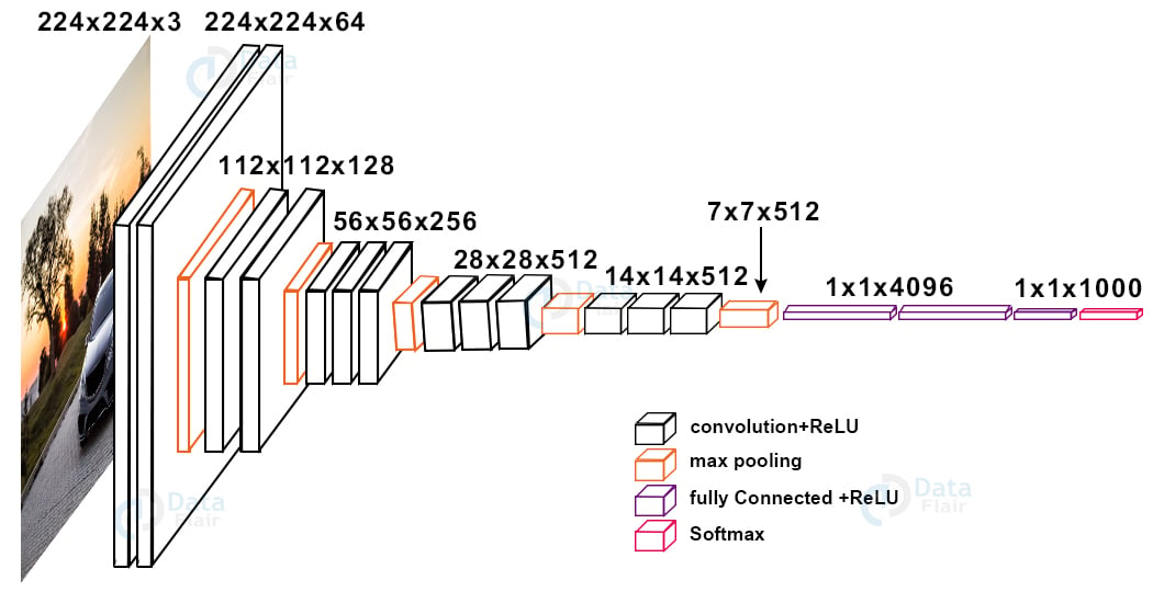
We remove the last layer of the VGG16 network and add layers that suit our problem.

from tensorflow.keras.layers import Input
from tensorflow.keras.layers import Dense
from tensorflow.keras.layers import AveragePooling2D
from tensorflow.keras.layers import Dropout
from tensorflow.keras.layers import Flatten
from tensorflow.keras.applications import VGG16

base_model = VGG16(weights= 'imagenet', input_tensor= Input(shape = (224, 224, 3)), include_top= False)
base_input = base_model.input

base_output = base_model.output
base_output = AveragePooling2D(pool_size=(4, 4))(base_output)
base_output = Flatten(name="flatten")(base_output)
base_output = Dense(64, activation="relu")(base_output)
base_output = Dropout(0.5)(base_output)
base_output = Dense(2, activation="softmax")(base_output)

Freeze the layers of our model. By doing this, the network is not trained from the very beginning. It uses the weights of previous layers and continues training for the layers we added on top of those layers. This reduces the training time by a drastic amount.

for layer in base_model.layers:
    layer.trainable = False

Now build the model and compile it using the Adam as optimizer with a learning rate of 0.001 and accuracy as metric. As we are building a binary classifier and the input is an image, binary cross entropy is used as a loss function.

from tensorflow.keras.models import Model
from tensorflow.keras.optimizers import Adam

model = Model(inputs = base_input, outputs = base_output)
model.compile(optimizer= Adam(learning_rate= 1e-3), metrics= ['accuracy'], loss= 'binary_crossentropy')

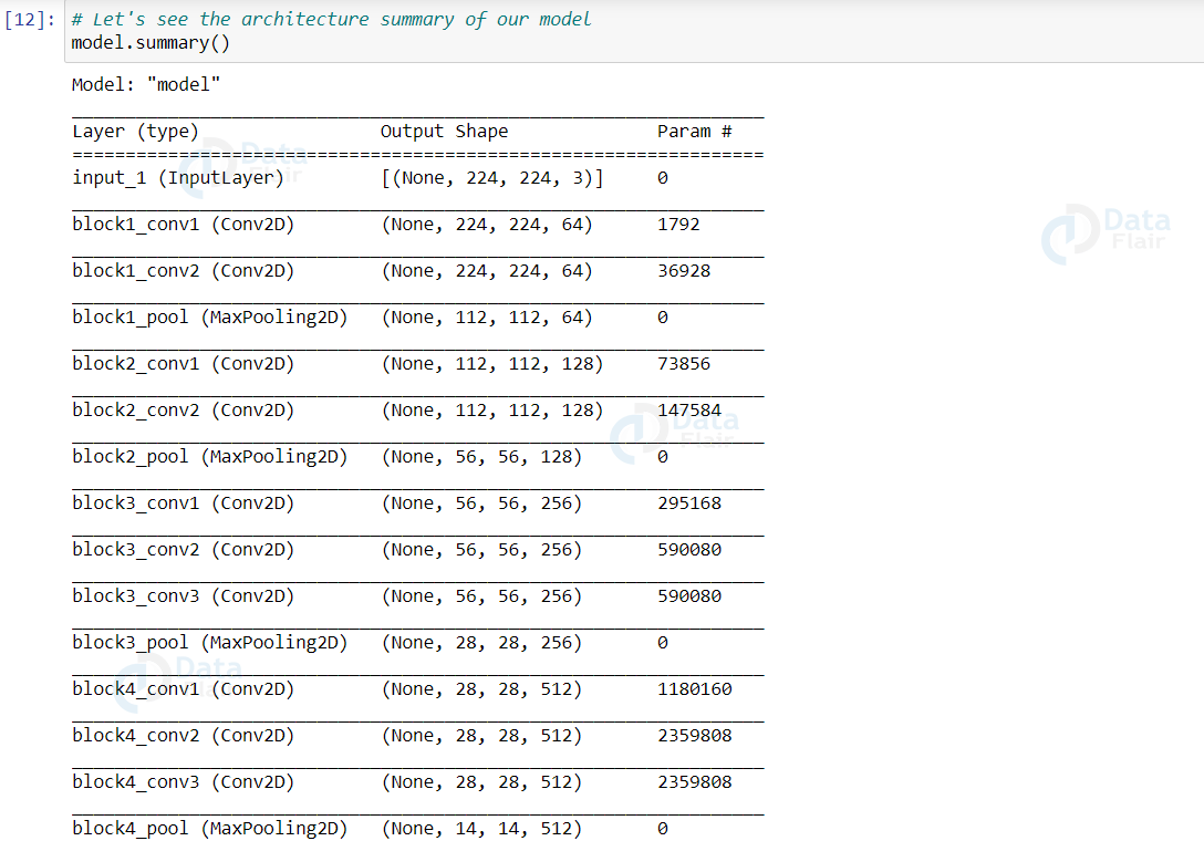
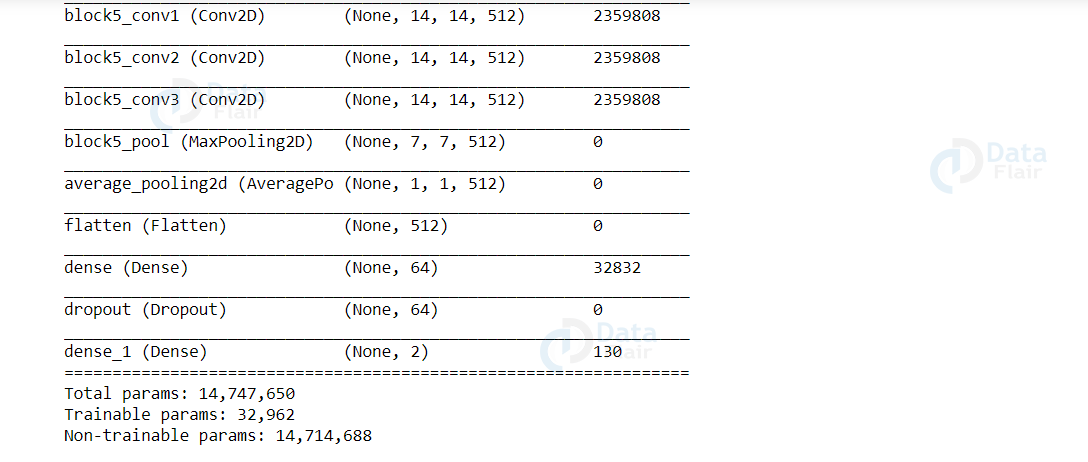
Now, let’s see the summary (architecture) of our model

model.summary()

Output:

Step 3: Train and evaluate the model

Before we start training our model, let’s store the following hyperparameters.

batch_size = 8
train_steps = len(train_X) // batch_size
validation_steps = len(test_X) // batch_size
epochs = 10

The model is trained on 10 epochs (full iterations) with train_steps for training set and validation_steps for validation set in each epoch. The batch size for each epoch is taken as 8.

Now, let’s train our model.

history = model.fit_generator(train_generator.flow(train_X, train_Y, batch_size= batch_size), steps_per_epoch= train_steps, validation_data = (test_X, test_Y), validation_steps= validation_steps, epochs= epochs)

Output:

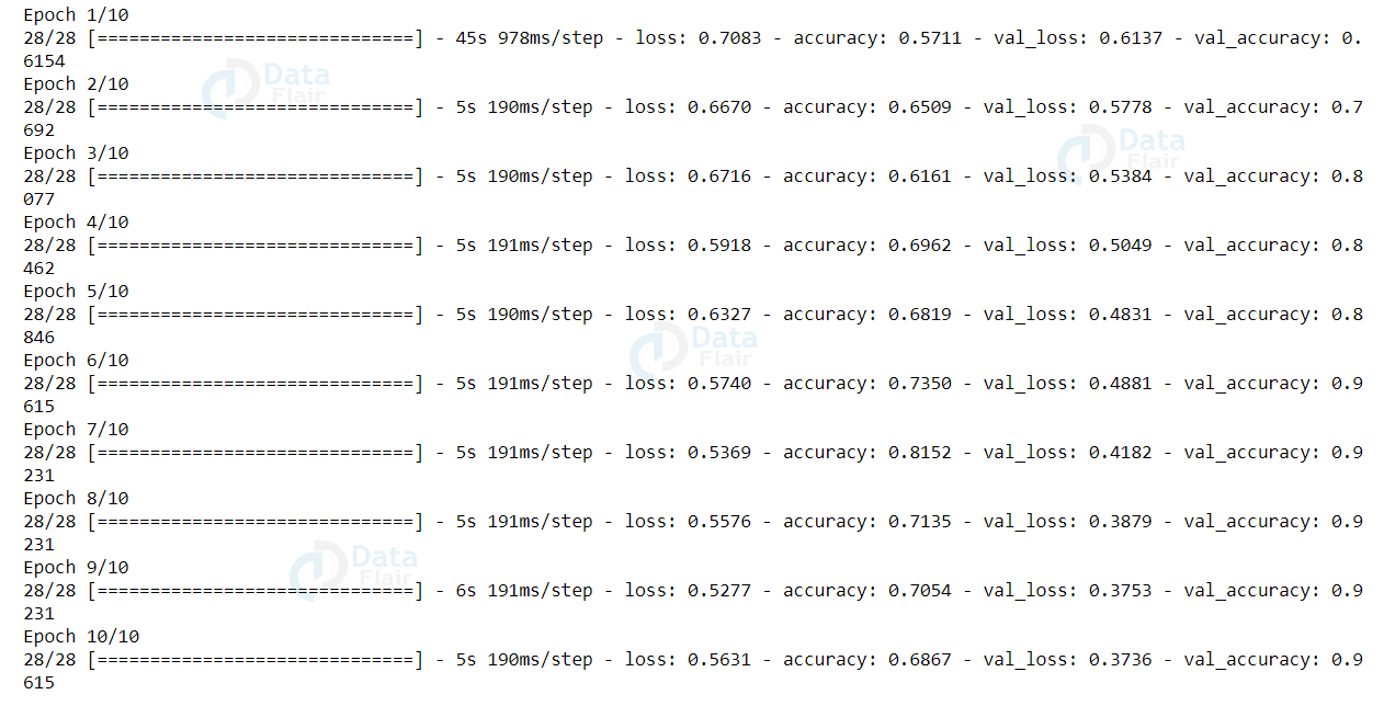
Our model got 96.5% accuracy on the test set. Now let’s evaluate our model using the predict() function.

from sklearn.metrics import classification_report, confusion_matrix

predictions = model.predict(test_X, batch_size= batch_size)
predictions = np.argmax(predictions, axis= 1)
actuals = np.argmax(test_Y, axis= 1)

print(classification_report(actuals, predictions, target_names= label_binarizer.classes_))

cm = confusion_matrix(actuals, predictions)
print(cm)

Output:

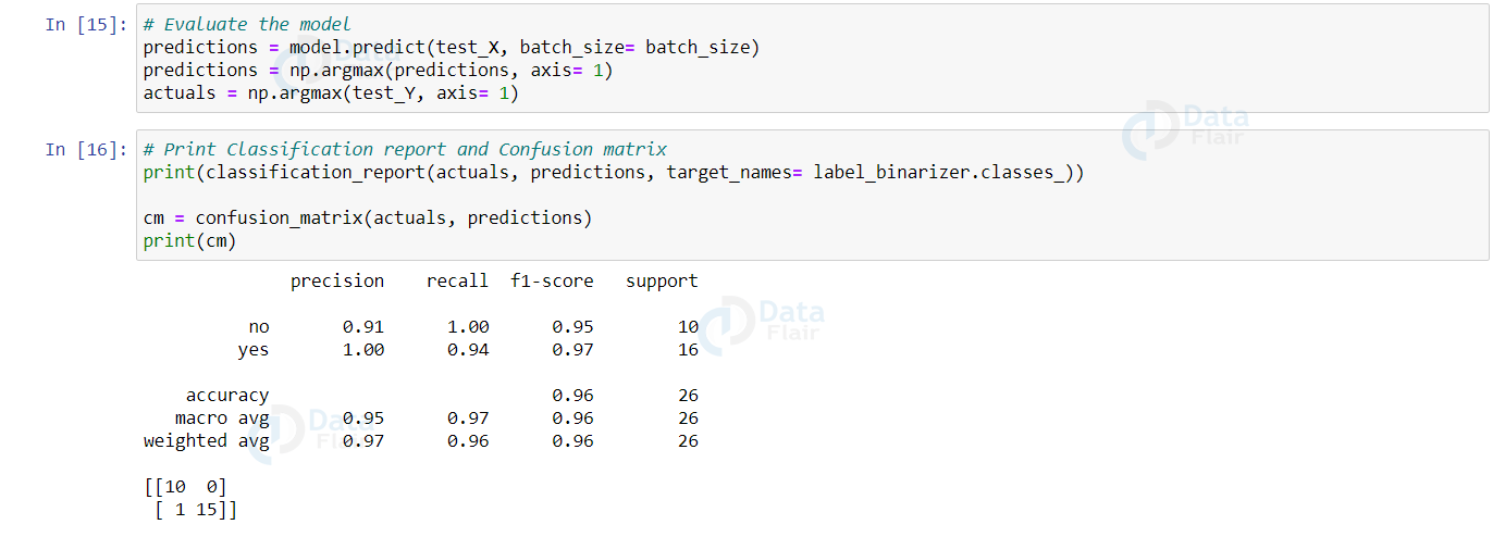
The predictions made by the model will be an array with each value being the probability that it predicts the image belongs to that category. So, we take the maximum of all such probabilities and assign the predicted label to that image input.

A confusion matrix is a matrix representation showing how well the trained model predicts each target class with respect to the counts. It contains 4 values in the following format:

TP FN
FP TN

• True positive (TP): Target is positive and the model predicted it as positive
• False negative (FN): Target is positive and the model predicted it as negative
• False positive (FP): Target is negative and the model predicted it as positive
• True negative (TN): Target is negative and the model predicted it as negative

The classification report provides a summary of the metrics precision, recall and F1-score for each class/label in the dataset. It also provides the accuracy and how many dataset samples of each label it categorized.

Now, let’s find the overall accuracy of the model using the formula: (TP + TN) / (TP + FN + FN + TN)

total = sum(sum(cm))
accuracy = (cm[0, 0] + cm[1, 1]) / total
print("Accuracy: {:.4f}".format(accuracy))

The accuracy of our model is found to be 96.15%

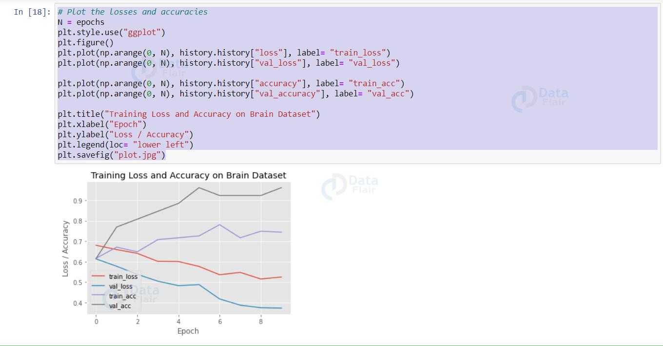
Using matplotlib, let’s plot the metrics.

N = epochs
plt.style.use("ggplot")
plt.figure()
plt.plot(np.arange(0, N), history.history["loss"], label= "train_loss")
plt.plot(np.arange(0, N), history.history["val_loss"], label= "val_loss")

plt.plot(np.arange(0, N), history.history["accuracy"], label= "train_acc")
plt.plot(np.arange(0, N), history.history["val_accuracy"], label= "val_acc")

plt.title("Training Loss and Accuracy on Brain Dataset")
plt.xlabel("Epoch")
plt.ylabel("Loss / Accuracy")
plt.legend(loc= "lower left")
plt.savefig("plot.jpg")

Output:

Summary

In brain tumor classification using machine learning, we built a binary classifier to detect brain tumors from MRI scan images. We built our classifier using transfer learning and obtained an accuracy of 96.5% and visualized our model’s overall performance.