In this blog, we will study Popular Search Algorithms in Artificial Intelligence. Also, we will lesrn all most popular techniques, methods, algorithms and searching techniques. We will use Popular Search Algorithms examples and images for the better understanding.
Introduction to Popular Search Algorithms in AI
In the artificial algorithm, to solve the problem we use the searching technique. The search algorithms help you to search for a particular position in such games.
Single Agent Pathfinding Problems
There are different types of games. Such as 3X3 eight-tile, 4X4 fifteen-tilepuzzles are single-agent-path-finding challenges. As they are consisting of a matrix of tiles with a blank tile.
Thus, to arrange the tiles by sliding a tile either vertically or horizontally into a blank space. Also, with the aim of accomplishing some objective.
Travelling Salesman Problem, Rubik’s Cube, and Theorem Proving
Search Algorithms Terminology
a. Problem Space
Basically, it is the environment in which the search takes place. (A set of states and set of operators to change those states)
b. Problem Instance
It is a result of Initial state + Goal state.
c. Problem Space Graph
We use it to represent problem state. Also, we use nodes to show states and operators are shown by edges.
d. The depth of a problem
We can define a length of the shortest path.
e. Space Complexity
We can calculate it as the maximum number of nodes that are stored in memory.
f. Time Complexity
It is defined as the maximum number of nodes that are created.
g. Admissibility
We can say it as a property of an algorithm that is used to find always an optimal solution.
h. Branching Factor
We can calculate it as the average number of child nodes in the problem space graph.
i. Depth
Length of the shortest path from an initial state to the goal state.
Brute-Force Search Strategies
This strategy doesn’t require any domain-specific knowledge. Thus it’s so simple strategy. Hence, it works very smoothly and fine with a small number of possible states.
Requirements for Brute Force Algorithms
b. A set of valid operators
d. Goal state description
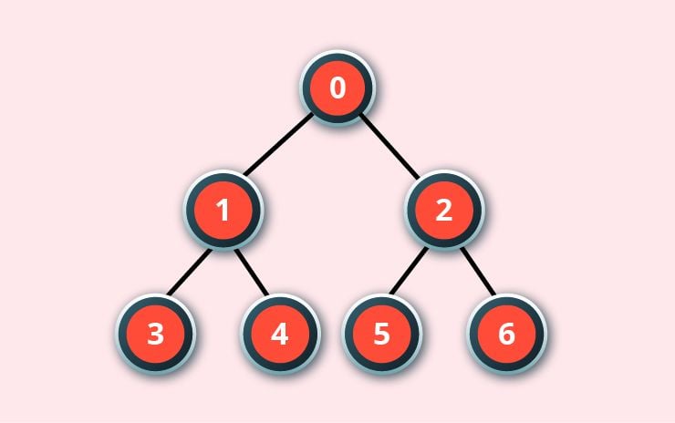
Breadth-First Search Algorithm in AI
Basically, we have to start searching for the root node. And continue through neighboring nodes first. Further, moves towards next level of nodes. Moreover, till the solution is found, generates one tree at a time.
As this search can be implemented using FIFO queue data structure. This method provides the shortest path to the solution.
FIFO(First in First Out).
If branching factor (average number of child nodes for a given node) = b and depth = d, the number of nodes at level d = bd.
The total no of nodes created in worst case is b + b2 + b3 + … + bd.
- It consumes a lot of memory space. As each level of nodes is saved for creating next one.
- Its complexity depends on the number of nodes. It can check duplicate nodes.

Breadth-First Search Algorithm
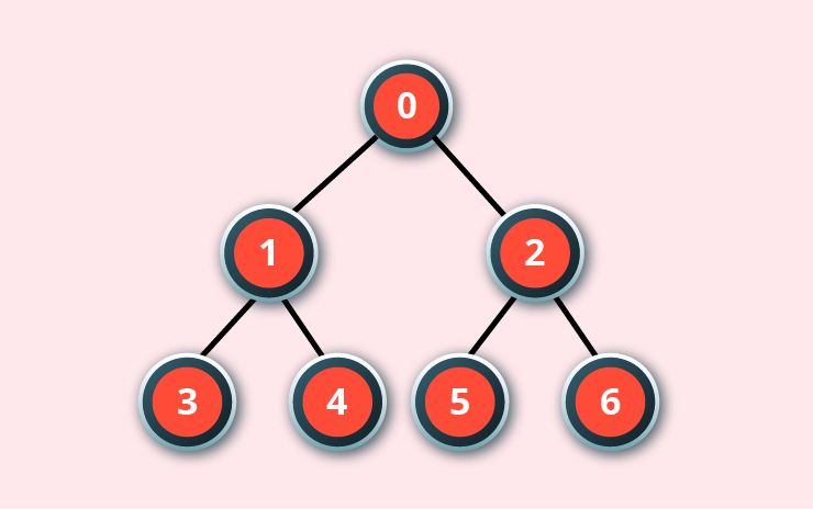
Depth-First Search Algorithm in AI
It is based on the concept of LIFO. As it stands for Last In First Out. Also, implemented in recursion with LIFO stack data structure. Thus, It used to create the same set of nodes as the Breadth-First method, only in the different order.
As the path is been stored in each iteration from root to leaf node. Thus, store nodes are linear with space requirement. With branching factor b and depth as m, the storage space is bm.
- As the algorithm may not terminate and go on infinitely on one path. Hence, a solution to this issue is to choose a cut-off depth.
- If the ideal cut-off is d, and if the chosen cut-off is lesser than d, then this algorithm may fail.
- If the chosen cut-off is more than d, then execution time increases.
- Its complexity depends on the number of paths. It cannot check duplicate nodes.
Depth-First Search Algorithm
Bidirectional Search Algorithm in AI
Basically, starts searches forward from an initial state and backward from goal state. As till both meets to identify a common state.
Moreover, initial state path is concatenated with the goal state inverse path. Each search is done only up to half of the total path.
Uniform Cost Search Algorithm in AI
- Basically, it performs sorting in increasing cost of the path to a node. Also, always expands the least cost node. Although, it is identical to Breadth-First search if each transition has the same cost.
- It explores paths in the increasing order of cost.
Disadvantage
- There can be multiple long paths with the cost ≤ C*.
- Uniform Cost search must explore them all.
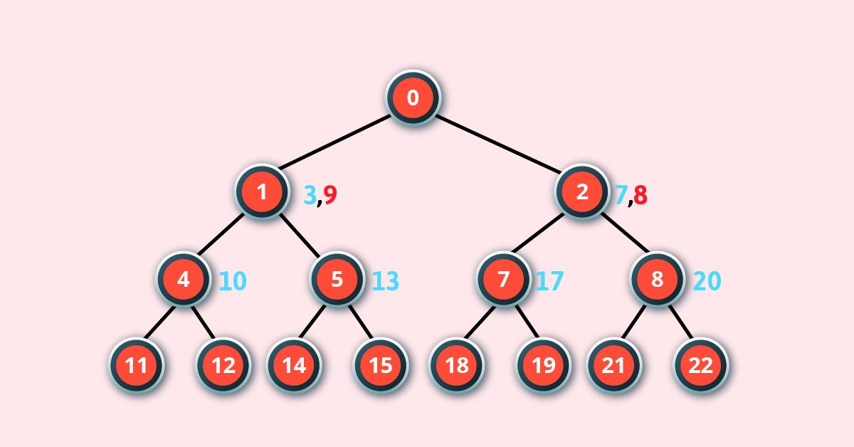
Iterative Deepening Depth-First Search Algorithm
To perform this search we need to follow steps. As it performs the DFS starting to level 1, starts and then executes a complete depth-first search to level 2.
Moreover, we have to continue searching process till we find the solution. We have to generate nodes till single nodes are created. Also, it saves only stack of nodes.
As soon as he finds a solution at depth d, the algorithm ends, The number of nodes created at depth d is bd and at depth d-1 is bd-1.
Iterative Deepening Depth-First Search Algorithm
Informed (Heuristic) Search Strategies Algorithm
To increase the efficiency of search algorithm we need to add problem-specific knowledge. We use this to solve large problems with large number of possible states
a. Heuristic Evaluation Functions
We use this function to calculate the path between two states that a function takes for sliding-tiles games. which we have to calculate by computing number of rows. Also, moves of each tile make from its goal state. Further, adding these number of moves for all tiles.
b. Pure Heuristic Search
In order, if heuristic value nodes will expand. Also, creates two lists:
- First, a closed list of the already expanded nodes;
- Secondly, an open list created. Although, unexpected nodes.
A node with a minimum heuristic value is expanded, In each iteration. Also, all its child nodes are created and placed on the closed list.
Further, we apply this heuristic function to child nodes. Thus, at last, we have to place it in the open list, as per the heuristic value. Although, we have to save the shortest path while to dispose of the longer ones.
A * Search Algorithm in AI
We can say that A * Search is the best form of Best First Search. Also, avoids expensive expanding path. Although, first expands most promising path.
f(n) = g(n) + h(n), where
g(n) is the cost to reach the node
h(n), it is estimated cost to get from the node to the goal
f(n) it is defined as the estimated total cost of path through n to goal. Also, we will use priority queue by increasing f(n) to implement it.
Greedy Best First Search Algorithm in AI
The node which is closest to goal will be expanded first. Although, explanation of nodes depends upon f(n) = h(n). Further, using priority queue we implement it.
Disadvantage
- It can get stuck in loops. It is not optimal.
Local Search Algorithms in AI
Basically, it’s Popular Search Algorithms. Also, a prospective solution. Further, moves to a neighboring solution. Moreover, returns a valid solution.
a. Hill-Climbing Search Algorithm in AI
We can start this algorithm with an arbitrary solution to a problem. Also, it’s an iterative algorithm. Hence, the algorithm attempts to better solution by single element of the solution.
Although, we take an incremental change as a new solution. As if the change produces a better solution. Moreover, we have to repeat until there are no further improvements.
As this function of the problem always, returns a state that is a local maximum.
inputs: problem, a problem
local variables: current, a node
current <-Make_Node(Initial-State[problem])
do neighbor <- a highest_valued successor of current
if Value[neighbor] ≤ Value[current] then
b. Local Beam Search Algorithm in AI
In this algorithm, we have to hold k number of states at any given time. At the beginning, we have to generated states randomly.
Moreover, with the objective function, we have to compute successors of these k states. Also, this stop, if any of these successors is the maximum value of the objective function.
Otherwise, we have to put the (initial k states and k number of successors of the states = 2k) states in a pool. Also, a pool is then sorted numerically. Further, we have to select highest k states as new initial states. This process continues until a maximum value is reached.
function BeamSearch( problem, k), returns a solution state.
start with k randomly generated states
generate all successors of all k states
if any of the states = solution, then return the state
else select the k best successors
Simulated Annealing Algorithm in AI
The process is of heating and cooling a metal to change its internal structure. Although, for modifying its physical properties is known as annealing. As soon as the metal cools, it forms a new structure.
Also, metal is going to retain its newly obtained properties. Although, we have to keep the variable temperature in a simulated annealing process.
First, we have to set high temperature. Then, left it to allow “cool” slowly with the proceeding algorithm. Further, if there is high temperature, algorithm accepts worse solutions with high frequency.
Start
Initialize k = 0; L = integer number of variables;
From i → j, search the performance difference Δ.
If Δ <= 0 then accept else if exp(-Δ/T(k)) > random(0,1) then accept;
Repeat steps 1 and 2 for L(k) steps.
Repeat steps 1 through 4 till the criteria matches.
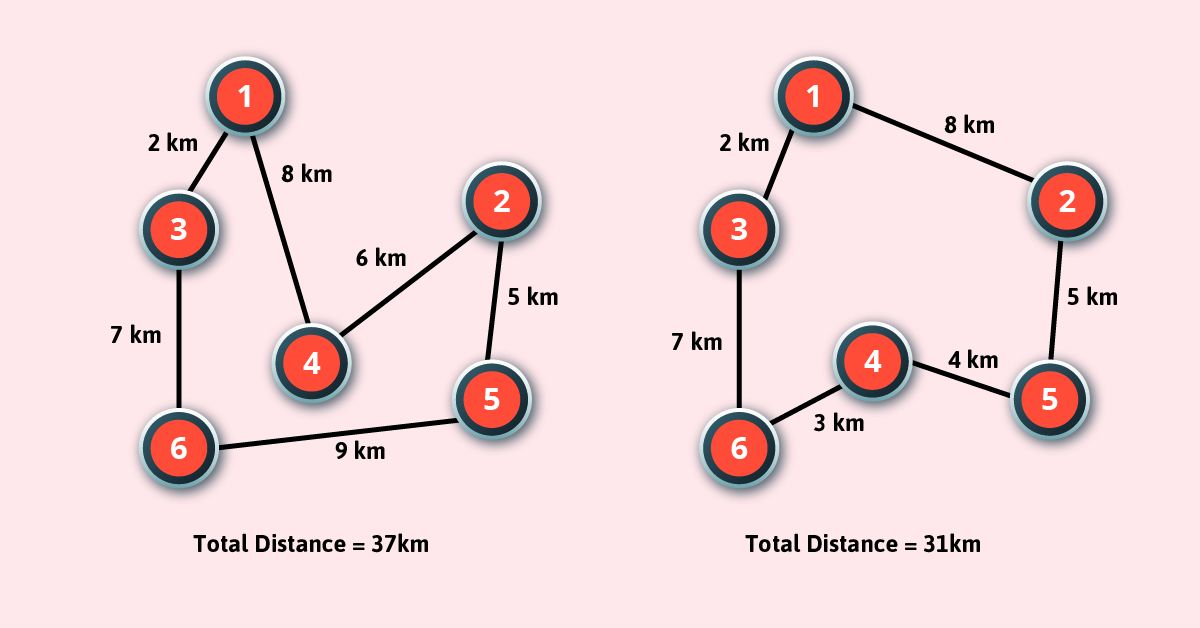
Travelling Salesman Problem
The main goal of this problem is to find a low-cost tour. That starts from a city, visits all cities en-route exactly once and ends at the same starting city.
Find out all (n -1)! Possible solutions, where n is the total number of cities.
Further, determine the minimum cost by finding out the cost of each of these (n -1)! solutions.
Finally, keep the one with the minimum cost.
Search algorithms help AI find answers. One popular algorithm is Breadth-First Search (BFS). It checks all possible paths one step at a time. It’s useful when all steps have equal cost, like finding the shortest path in a maze. BFS is simple but takes more memory.
Depth-First Search (DFS) goes deep into one path before trying others. It’s like following one road fully, then coming back to try the next. DFS is memory-efficient but can get stuck going too deep. Both BFS and DFS are used in problem-solving and pathfinding.
Another powerful search method is A* (A-Star) algorithm. It combines the best of BFS and heuristics. A* finds the shortest path by choosing the most promising path first. It is used in GPS systems, games, and robots. Search algorithms help AI find the best solutions in the smartest way.
Furthermore, if you feel any query to understand Popular Search Algorithms, then feel free to ask in the comment section.