Keras Convolution Neural Network Layers and Working

We widely use Convolution Neural Networks for computer vision and image classification tasks. The Convolution Neural Network architecture generally consists of two parts. The first part is the feature extractor which we form from a series of convolution and pooling layers. The second part includes fully connected layers which act as classifiers.

In this article, we will study how to use Convolution Neural Networks for image classification tasks. We will walk through a few examples to show the code for the implementation of Convolution Neural Networks in Keras.

Convolution Neural Network Architecture

The convolution neural network algorithm is the result of continuous advancements in computer vision with deep learning.
CNN is a Deep learning algorithm that is able to assign importance to various objects in the image and able to differentiate them.
CNN has the ability to learn the characteristics and perform classification.
An input image has many spatial and temporal dependencies, CNN captures these characteristics using relevant filters/kernels.

A Kernel or filter is an element in CNN that performs convolution around the image in the first part. The kernel moves to the right and shifts according to the stride value. Every time during convolution a matrix multiplication operation is performed.

After convolution, we obtain another image with a different height, width, and depth. We obtain more channels than just RGB but less width and height.

We slide each filter though out the image step by step, this step in the forward pass is called stride.

Layers in CNN

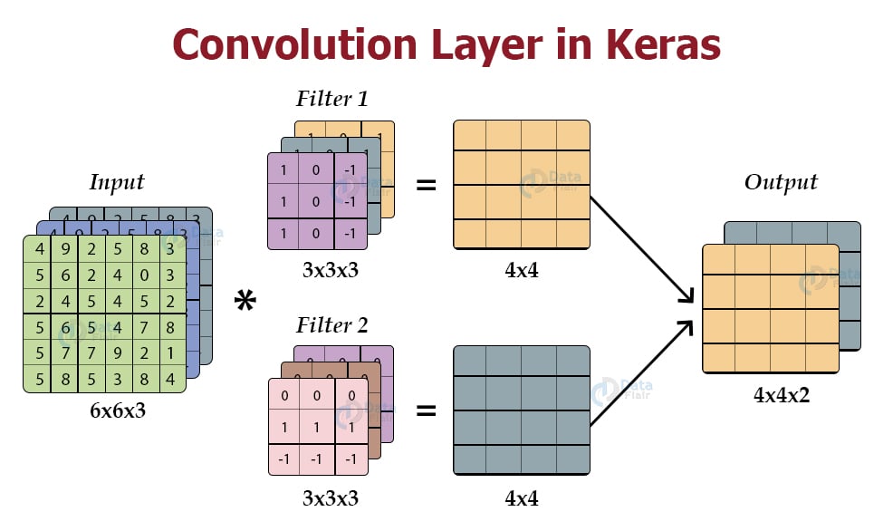
1. Keras Convolution layer

It is the first layer to extract features from the input image. Here we define the kernel as the layer parameter. We perform matrix multiplication operations on the input image using the kernel.

Example:

Suppose a 3*3 image pixel and a 2*2 filter as shown:

pixel : [[1,0,1],
[0,1,0],
[1,0,1]]
filter : [[1,0],
[0,1]]

The restaurant matrix after convolution of filter would be:
[[2,0],
[0,2]]

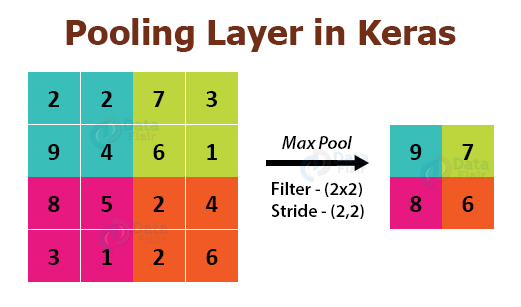
2. Keras Pooling Layer

After convolution, we perform pooling to reduce the number of parameters and computations.
There are different types of pooling operations, the most common ones are max pooling and average pooling.

Example:
Take a sample case of max pooling with 2*2 filter and stride 2.

Image pixels:
[[1,2,3,4],
[5,6,7,8],
[3,4,5,6],
[6,7,8,9]]

The resultant matrix after max-pooling would be:
[[6,8],
[7,9]]

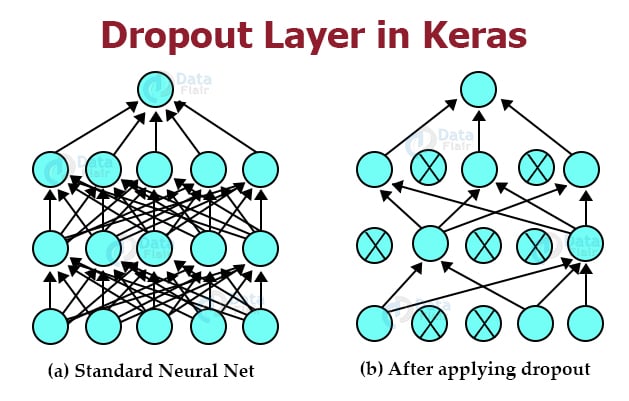
3. Keras Dropout Layer

It is used to prevent the network from overfitting. In this layer, some fraction of units in the network is dropped in training such that the model is trained on all the units.

A series of convolution and pooling layers are used for feature extraction. After that, we construct densely connected layers to perform classification based on these features.

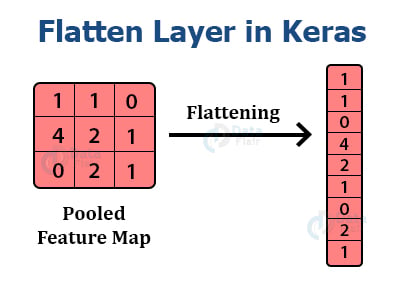
4. Keras Flatten Layer

It is used to convert the data into 1D arrays to create a single feature vector. After flattening we forward the data to a fully connected layer for final classification.

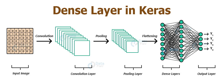
5. Keras Dense Layer

It is a fully connected layer. Each node in this layer is connected to the previous layer i.e densely connected. This layer is used at the final stage of CNN to perform classification.

Implementing CNN on CIFAR 10 Dataset

CIFAR 10 dataset consists of 10 image classes. The available image classes are :

• Car
• Airplane
• Bird
• Cat
• Deer
• Dog
• Frog
• Horse
• Ship
• Truck

This is one of the most popular datasets that allow researchers to practice different algorithms for object recognition.
Convolution Neural Networks have shown the best results in solving the CIFAR-10 problem.

Let’s build our Convolution model to recognize CIFAR-10 classes.

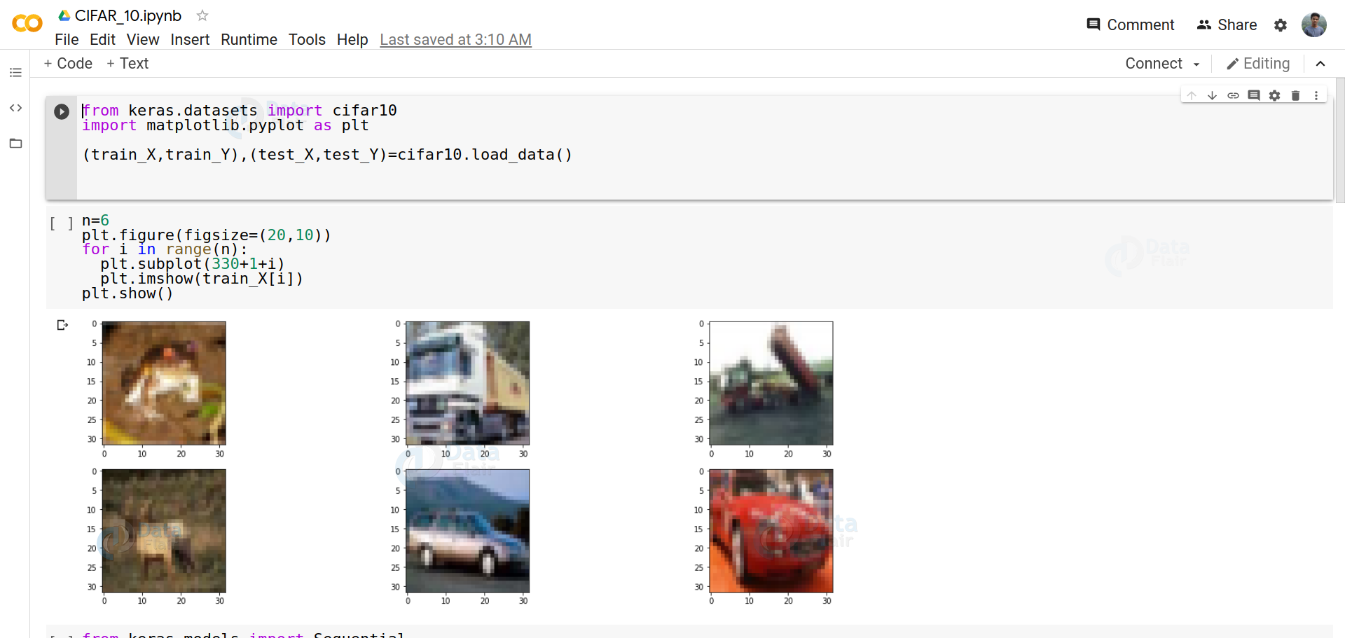
1. Load the dataset from keras datasets module.

from keras.datasets import cifar10
import matplotlib.pyplot as plt

(train_X,train_Y),(test_X,test_Y)=cifar10.load_data()

2. To visualize the dataset

n=6
plt.figure(figsize=(20,10))
for i in range(n):
plt.subplot(330+1+i)
plt.imshow(train_X[i])
plt.show()

3. The dataset looks like

Now import required modules,

from keras.models import Sequential
from keras.layers import Dense
from keras.layers import Dropout
from keras.layers import Flatten
from keras.constraints import maxnorm
from keras.optimizers import SGD
from keras.layers.convolutional import Conv2D
from keras.layers.convolutional import MaxPooling2D
from keras.utils import np_utils

4. Normalizing inputs

train_x=train_X.astype('float32')
test_X=test_X.astype('float32')

train_X=train_X/255.0
test_X=test_X/255.0

5. One hot encoding

train_Y=np_utils.to_categorical(train_Y)
test_Y=np_utils.to_categorical(test_Y)

num_classes=test_Y.shape[1]

6. Build the model

model=Sequential()
model.add(Conv2D(32,(3,3),input_shape=(32,32,3),padding='same',activation='relu',kernel_constraint=maxnorm(3)))
model.add(Dropout(0.2))
model.add(Conv2D(32,(3,3),activation='relu',padding='same',kernel_constraint=maxnorm(3)))
model.add(MaxPooling2D(pool_size=(2,2)))
model.add(Flatten())
model.add(Dense(512,activation='relu',kernel_constraint=maxnorm(3)))
model.add(Dropout(0.5))
model.add(Dense(num_classes, activation='softmax'))

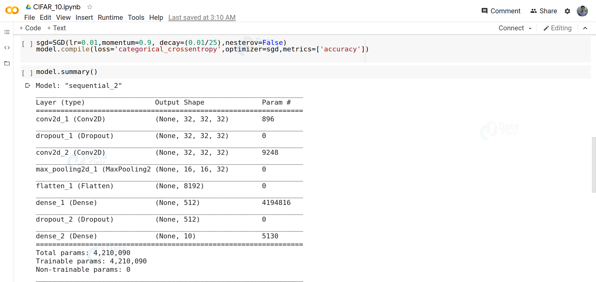
7. Model Compiling

sgd=SGD(lr=0.01,momentum=0.9, decay=(0.01/25),nesterov=False)
model.compile(loss='categorical_crossentropy',optimizer=sgd,metrics=['accuracy'])

8. Analyzing Model Summary

model.summary()

9. Train the model and check its accuracy on test data

model.fit(train_X,train_Y,validation_data=(test_X,test_Y),epochs=10,batch_size=32)

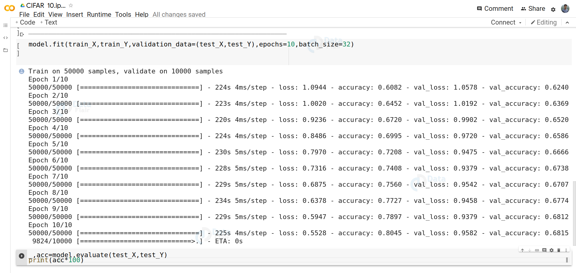
10. Evaluate the model

_,acc=model.evaluate(test_X,test_Y)
print(acc*100)

Implementing CNN on Fashion MNIST Dataset

The Fashion MNIST dataset consists of a training set of 60000 images and a testing set of 10000 images. There are 10 image classes in this dataset and each class has a mapping corresponding to the following labels:

• 0 T-shirt/top
• 1 Trouser
• 2 pullover
• 3 Dress
• 4 Coat
• 5 sandals
• 6 shirt
• 7 sneaker
• 8 bag
• 9 ankle boot

Let’s build our CNN model on this dataset.

1. Import required modules

from numpy import mean
from numpy import std
from matplotlib import pyplot
from sklearn.model_selection import KFold
from keras.datasets import fashion_mnist
from keras.utils import to_categorical
from keras.models import Sequential
from keras.layers import Conv2D
from keras.layers import MaxPooling2D
from keras.layers import Dense
from keras.layers import Flatten
from keras.optimizers import SGD

2. Load the dataset

(train_X,train_Y),(test_X,test_Y)=fashion_mnist.load_data()

3. Reshaping and one hot encoding

train_X=train_X.reshape((train_X.shape[0],28,28,1))
test_X=test_X.reshape((test_X.shape[0],28,28,1))

train_Y=to_categorical(train_Y)
test_Y=to_categorical(test_Y)

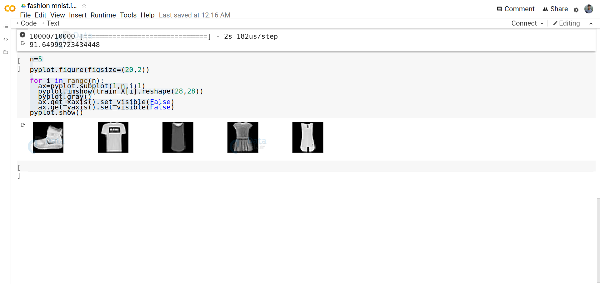
4. Visualize the dataset using matplotlib

n=5

pyplot.figure(figsize=(20,2))

for i in range(n):
ax=pyplot.subplot(1,n,i+1)
pyplot.imshow(train_X[i].reshape(28,28))
pyplot.gray()
ax.get_xaxis().set_visible(False)
ax.get_yaxis().set_visible(False)
pyplot.show()

5. Normalizing data

train_X=train_X.astype('float32')
test_X=test_X.astype('float32')

train_X=train_X/255.0
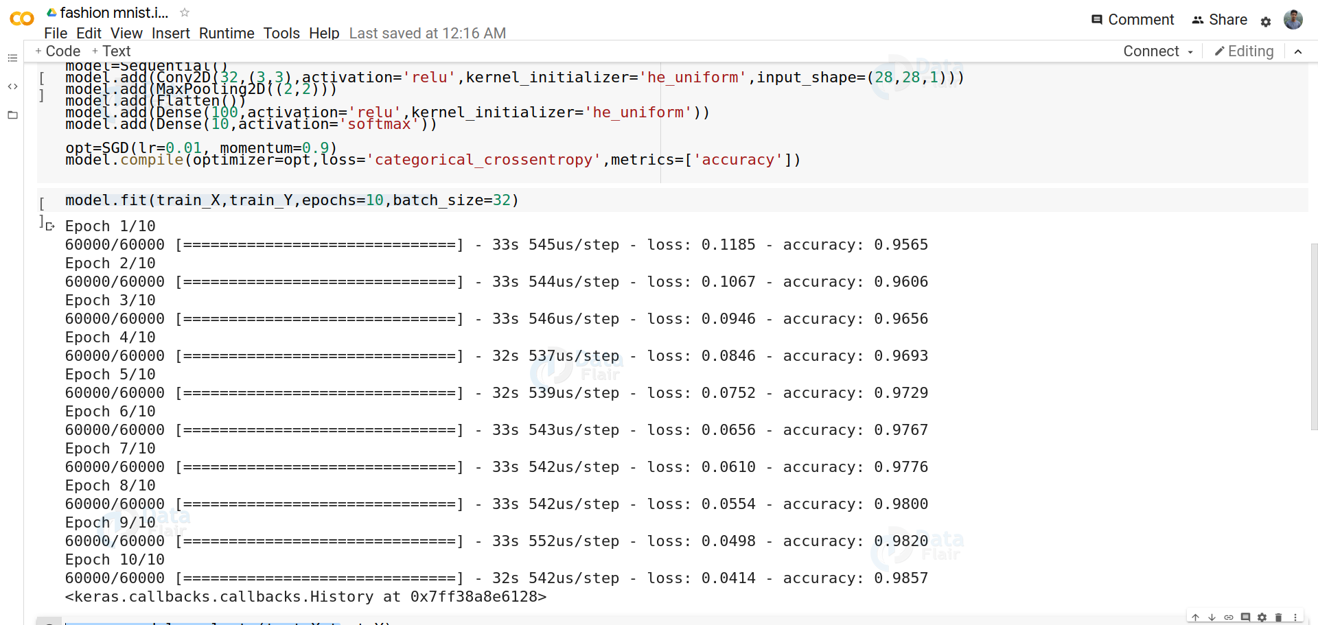
test_X=test_X/255.0

6. Build the model

model=Sequential()
model.add(Conv2D(32,(3,3),activation='relu',kernel_initializer='he_uniform',input_shape=(28,28,1)))
model.add(MaxPooling2D((2,2)))
model.add(Flatten())
model.add(Dense(100,activation='relu',kernel_initializer='he_uniform'))
model.add(Dense(10,activation='softmax'))

opt=SGD(lr=0.01, momentum=0.9)
model.compile(optimizer=opt,loss='categorical_crossentropy',metrics=['accuracy'])

7. Training our model

model.fit(train_X,train_Y,epochs=10,batch_size=32)

8. Evaluate our Model P

erformance

_, acc=model.evaluate(test_X,test_Y)
print(acc*100)

Summary

This tutorial talks about the use of cases of convolution neural network and explains how to implement them in Keras. Convolution Neural Networks have outstanding results on image classification problems. The above examples verify this fact. Here we have shown two examples of Convolution Neural Network – One on CIFAR 10 dataset problem and another on Fashion MNIST dataset problem.