OpenCV Morphological Operations

Step into the realm where pixels transform into artistry, where shapes hold secrets, and where the essence of images is refined through a digital touch.

In the world of image processing, there exists a fascinating toolkit known as ‘morphological operations. Much like an artisan shaping clay into intricate forms, morphological operations sculpt and refine images based on their structure and contours.

These operations, often employed in fields from medicine to machine vision, possess the power to unveil hidden patterns, enhance edges, and blur the line between reality and digital interpretation.

In this journey, we delve into the wonders of morphological operations, exploring their fundamental techniques, unmasking their applications, and uncovering the art of reshaping visual insights.

Opening Operation in OpenCV: Unveiling Image Enhancement

In the arsenal of morphological operations, the “opening” operation stands as a versatile tool for image enhancement and noise reduction. OpenCV, a powerhouse library for computer vision, provides a straightforward way to implement this operation using the `cv2.morphologyEx()` function. This section uncovers the inner workings of the opening operation, dissecting its syntax, parameters, and accompanying code.

Syntax :

cv2.morphologyEx(src, op, kernel, dst, anchor, iterations, borderType, borderValue)

Parameters :

• Src: The source image is usually a grayscale or binary image.
• Op: The morphological operation to be performed. In this case, it should be cv2.MORPH_OPEN for the opening operation.
• Kernel: The operational, structural element that establishes the neighborhood’s size and shape.
• Dst: The optional destination image where the result is stored.
• Anchor: The anchor point within the kernel. If negative, it’s considered the centre.
• Iterations: The number of times the operation is applied. The default is 1.
• borderType: The pixel extrapolation method.
• borderValue: The value used for padding in case of borderType.

Code with Explanation :

import cv2
import numpy as np

# Load the source image
src_image = cv2.imread(r"C:\Users\Satchit\OneDrive\Desktop\OpenCV DataFlair\MorphologicalOperations\wildlife-leopard.jpg",cv2.IMREAD_GRAYSCALE)

# Define the kernel (structuring element) for the opening operation
kernel = np.ones((5, 5), np.uint8)

# Apply the opening operation using cv2.morphologyEx()
opened_image = cv2.morphologyEx(src_image, cv2.MORPH_OPEN, kernel)

# Display the original and opened images
cv2.imshow('Original Image', src_image)
cv2.imshow('Opened Image', opened_image)
cv2.waitKey(0)
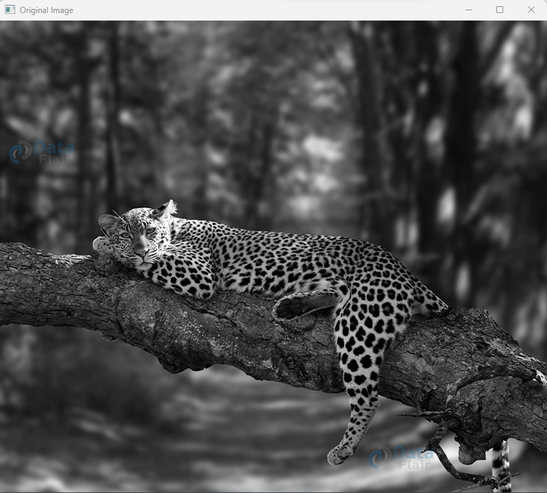
cv2.destroyAllWindows()

Original Image :

Opened Image :

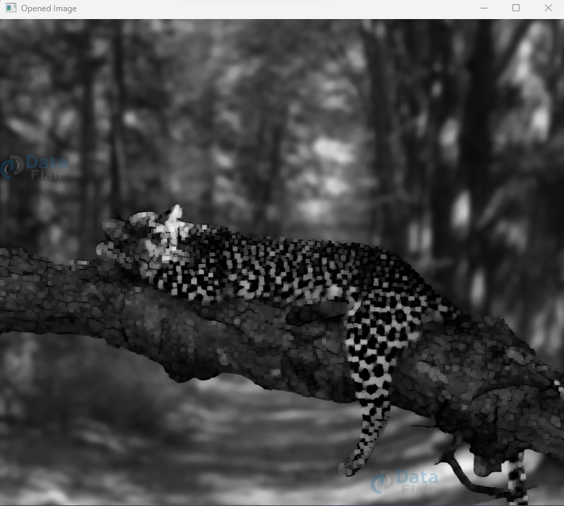
Explanation :

1. We begin by loading the source image in grayscale using cv2.imread() with the cv2.IMREAD_GRAYSCALE flag.

2. A suitable kernel is defined using np.ones() with a size of (5, 5), implying a 5×5 rectangular structuring element. You can adjust the kernel size based on your specific requirements.

3. The cv2.morphologyEx() function is invoked, where we pass the source image, the cv2.MORPH_OPEN operation, and the defined kernel.

4. The result, the opened image, is stored in the `opened_image` variable.

5. Using cv2.imshow(), we display both the original and opened images, allowing a visual comparison.

The opening operation effectively erodes and then dilates the image, which helps eliminate small noise while preserving the larger structures. This process can be fine-tuned by adjusting the kernel size and other parameters to suit the characteristics of the image you’re working with.

Closing Operation in OpenCV: Sealing Image Enhancements

Continuing our exploration of morphological operations, we turn our attention to the “closing” operation – a technique that fills gaps and completes fragmented elements within an image. OpenCV, the stalwart of computer vision libraries, provides a seamless way to implement the closing operation through the `cv2.morphologyEx()` function. In this section, we uncover the essence of the closing operation, delving into its syntax, parameters, and accompanying code.

Syntax :

cv2.morphologyEx(src, op, kernel, dst, anchor, iterations, borderType, borderValue)

Parameters :

• Src: The source image, typically in grayscale or binary format.
• Op: Denotes the morphological operation to be performed, here, it should be set to cv2.MORPH_CLOSE for the closing operation.
• Kernel: Defines the structuring element that determines the shape and size of the local neighborhood.
• Dst: An optional destination image where the result will be stored.
• Anchor: Specifies the anchor point within the kernel. A negative value indicates the centre.
• Iterations: Dictates how many times the operation is applied. The default value is 1.
• borderType: Determines the pixel extrapolation method.
• borderValue: Sets the value used for padding when applying the borderType.

Code with Explanation :

import cv2
import numpy as np

# Load the source image
src_image = cv2.imread(r"C:\Users\Satchit\OneDrive\Desktop\OpenCV DataFlair\MorphologicalOperations\wildlife-leopard.jpg",cv2.IMREAD_GRAYSCALE)
# Define the kernel (structuring element) for the closing operation
kernel = np.ones((5, 5), np.uint8)

# Apply the closing operation using cv2.morphologyEx()
closed_image = cv2.morphologyEx(src_image, cv2.MORPH_CLOSE, kernel)
# Display the original and closed images
cv2.imshow('Original Image', src_image)
cv2.imshow('Closed Image', closed_image)
cv2.waitKey(0)
cv2.destroyAllWindows()

Original Image :

Closed Image :

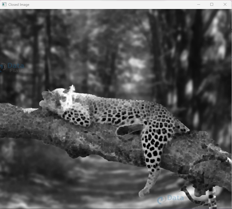
Explanation :

1. We initiate by loading the source image in grayscale using cv2.imread() and specifying the cv2.IMREAD_GRAYSCALE flag.

2. The kernel, representing the structuring element, is created using np.ones() with dimensions (5, 5), forming a 5×5 rectangular structure. Adjust the kernel size based on your specific needs.

3. The cv2.morphologyEx() function is invoked with the source image, the cv2.MORPH_CLOSE operation, and the defined kernel being passed as arguments.

4. The result, the closed image, is stored in the variable closed_image.

5. We use cv2.imshow() to present both the original and closed images, enabling a visual comparison.

The closing operation, achieved by first dilating and then eroding the image, helps bridge gaps and complete fragmented structures. Customizing the kernel size and other parameters allows you to tailor the operation to the characteristics of the image you’re working with, achieving optimal results in noise reduction and enhancing object connectivity.

Morphological Gradient in OpenCV: Revealing Object Boundaries

Embark on a journey into the intricate world of image processing as we unravel the concept of the “morphological gradient.” This technique serves as a remarkable tool for highlighting object boundaries within images, offering insights into their contours and shapes.

OpenCV, the cornerstone of computer vision libraries, introduces the `cv2.morphologyEx()` function as a gateway to implementing the morphological gradient. In this section, we unveil the essence of the morphological gradient, dissecting its syntax, parameters, and accompanying code.

Syntax :

cv2.morphologyEx(src, op, kernel, dst, anchor, iterations, borderType, borderValue)

Parameters :

• Src: The source image, often in grayscale or binary form.
• Op: Specifies the morphological operation to be performed. For the morphological gradient, set op to cv2.MORPH_GRADIENT.
• Kernel: Defines the structuring element, determining the shape and size of the local area.
• Dst: An optional destination image to store the result.
• anchor: Determines the anchor point within the kernel. A negative value denotes the centre.
• iterations: Dictates the number of times the operation is applied. The default is 1.
• borderType: Chooses the pixel extrapolation method.
• borderValue: Sets the value used for padding in cases where borderType is applied.

Code with Explanation :

import cv2
import numpy as np

# Load the source image
src_image = cv2.imread(r"C:\Users\Satchit\OneDrive\Desktop\OpenCV DataFlair\MorphologicalOperations\wildlife-leopard.jpg",cv2.IMREAD_GRAYSCALE)


# Define the kernel (structuring element) for the morphological gradient
kernel = np.ones((5, 5), np.uint8)

# Apply the morphological gradient using cv2.morphologyEx()
gradient_image = cv2.morphologyEx(src_image, cv2.MORPH_GRADIENT, kernel)

# Display the original and gradient images
cv2.imshow('Original Image', src_image)
cv2.imshow('Gradient Image', gradient_image)
cv2.waitKey(0)
cv2.destroyAllWindows()

Original Image :

Gradient Image :

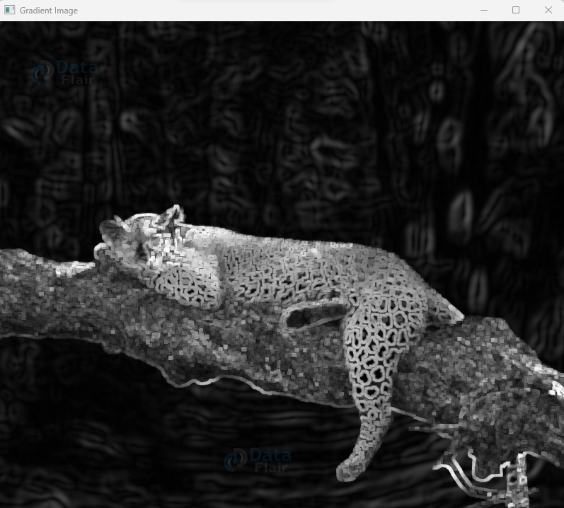
Explanation :

1. We initiate the process by loading the source image in grayscale using cv2.imread() and specifying the cv2.IMREAD_GRAYSCALE flag.

2. A kernel, representing the structuring element, is created using np.ones() with dimensions (5, 5), forming a 5×5 rectangular structure. Adjust the kernel size to match your requirements.

3. The cv2.morphologyEx() function is invoked with the source image, cv2.MORPH_GRADIENT operation, and the defined kernel being passed as arguments.

4. The resulting image, the morphological gradient, is stored in the gradient_image variable.

5. To visualize the process, we use cv2.imshow() to display both the original and gradient images, facilitating a visual comparison.

The morphological gradient operation effectively captures the variations in intensity across object boundaries. By subtracting the erosion of the image from its dilation, this technique accentuates the edges and contours of objects, rendering them more prominent. Adjusting the kernel size and other parameters allows you to fine-tune the operation to best suit your image analysis needs.

Top Hat and Black Hat Morphological Operations in OpenCV: Illuminating Image Details

Venture deeper into the realm of image processing as we uncover the intriguing world of “Top Hat” and “Black Hat” morphological operations. These operations, often referred to as complementary pairings, are designed to enhance subtle image details that might otherwise remain concealed.

OpenCV, the bedrock of computer vision libraries, provides a seamless gateway through the `cv2.morphologyEx()` function to execute these operations. In this section, we delve into the heart of Top Hat and Black Hat operations, deconstructing their syntax, parameters, and accompanying code.

Syntax:

cv2.morphologyEx(src, op, kernel, dst, anchor, iterations, borderType, borderValue)

Parameters :

• Src: The source image, typically in grayscale or binary form.
• Op: Specifies the morphological operation to be performed – either cv2.MORPH_TOPHAT for Top Hat or cv2.MORPH_BLACKHAT for Black Hat.
• Kernel: Defines the structuring element, determining the shape and size of the local neighborhood.
• Dst: An optional destination image to hold the result.
• anchor: Specifies the anchor point within the kernel. A negative value denotes the centre.
• Iterations: Dictates the number of times the operation is applied. The default is 1.
• borderType: Determines the pixel extrapolation method.
• borderValue: Sets the value used for padding in cases where `borderType` is applied.

Code with Explanation (Top Hat Operation ) :

import cv2
import numpy as np

# Load the source image
src_image = cv2.imread(r"C:\Users\satchit\OneDrive\Desktop\OpenCV Data Flair\MorphologicalOperations\wildlife-leopard.jpg",cv2.IMREAD_GRAYSCALE)
# Define the kernel (structuring element) for the Top Hat operation
kernel = np.ones((5, 5), np.uint8)

# Apply the Top Hat operation using cv2.morphologyEx()
tophat_image = cv2.morphologyEx(src_image, cv2.MORPH_TOPHAT, kernel)
# Display the original and Top Hat images
cv2.imshow('Original Image', src_image)
cv2.imshow('Top Hat Image', tophat_image)
cv2.waitKey(0)
cv2.destroyAllWindows()

Original Image :

Top Hat Image :

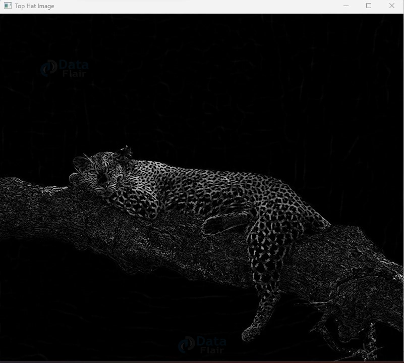
Explanation :

1. Start by loading the source image in grayscale using cv2.imread() with the cv2.IMREAD_GRAYSCALE flag.

2. Define the kernel (structuring element) using np.ones() with dimensions (5, 5), forming a 5×5 rectangular structure. Adjust the kernel size to match your needs.

3. Invoke cv2.morphologyEx() with the source image, cv2.MORPH_TOPHAT operation, and the defined kernel.

4. Store the outcome, the Top Hat image, in the variable tophat_image.

5. Visualize the transformation by using cv2.imshow() to showcase both the original and Top Hat images.

The Top Hat operation, achieved by subtracting the opening operation from the original image, effectively emphasizes fine details, such as small objects and textures. By adjusting the kernel size and other parameters, you can tailor the operation to bring forth specific details that are of interest in your image analysis.

Code with Explanation (Black Hat Operation) :

import cv2
import numpy as np

# Load the source image
src_image = cv2.imread(r"C:\Users\Satchit\OneDrive\Desktop\OpenCV DataFlair\MorphologicalOperations\wildlife-leopard.jpg",cv2.IMREAD_GRAYSCALE)

# Define the kernel (structuring element) for the Black Hat operation
kernel = np.ones((5, 5), np.uint8)

# Apply the Black Hat operation using cv2.morphologyEx()
blackhat_image = cv2.morphologyEx(src_image, cv2.MORPH_BLACKHAT, kernel)

# Display the original and Black Hat images
cv2.imshow('Original Image', src_image)
cv2.imshow('Black Hat Image', blackhat_image)
cv2.waitKey(0)
cv2.destroyAllWindows()

Original Image :

Black Hat Image :

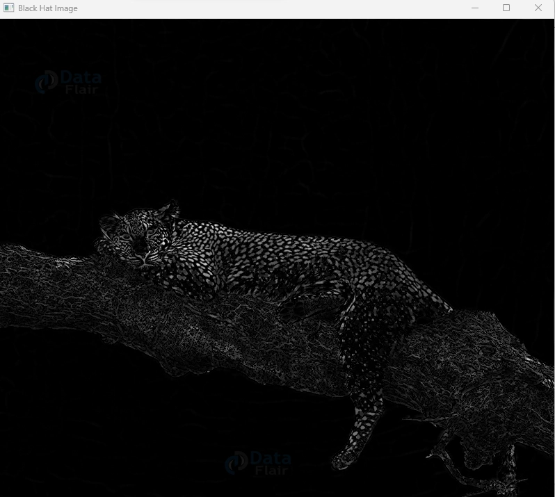
Explanation :

1. Begin by loading the source image in grayscale using cv2.imread() with the cv2.IMREAD_GRAYSCALE flag.

2. Define the kernel (structuring element) using np.ones() with dimensions (5, 5), forming a 5×5 rectangular structure. Adjust the kernel size as needed.

3. Utilize cv2.morphologyEx() with the source image, cv2.MORPH_BLACKHAT operation, and the defined kernel.

4. Store the outcome, the Black Hat image, in the variable blackhat_image.

5. Visualize the transformation by using cv2.imshow() to display both the original and Black Hat images.

By removing the closure process from the original image, the Black Hat operation successfully draws attention to regions of interest that stand out dramatically from their surroundings. This might be helpful for spotting abnormalities or emphasizing areas in an image with peculiar characteristics. You can adapt the procedure to your unique picture analysis objectives by adjusting the kernel size and other parameters.

Summary

In the captivating domain of image manipulation, the allure of morphological operations shines brightly. Through dilation, erosion, opening, closing, and advanced techniques like morphological gradient, Top Hat, and Black Hat operations, images undergo remarkable transformations.

These operations, like skilled artisans, refine images by enhancing features, eradicating noise, and revealing hidden structures. Their influence spans diverse fields, from medical diagnostics to industrial automation, infusing clarity and precision.

As our journey ends, remember that every parameter tweak or operation choice opens a new window into an image’s essence. OpenCV Morphological operations merge artistry and science, empowering you to sculpt visual narratives that transcend pixels, telling stories that echo far beyond the digital canvas.