Image Thresholding in OpenCV

Unravel the hidden patterns within images and unlock the magic of image segmentation with the power of Thresholding in OpenCV. From transforming grayscale wonders into clear-cut binary visions to conquering complex computer vision challenges.

This article will guide you through the art of Thresholding, offering insights into its versatile techniques and applications. Get ready to witness the visual world through a new lens as we delve into the captivating realm of Thresholding magic!

Thresholding, in simple words, is a technique used in image processing to convert a grayscale or color image into a binary image. It involves setting a specific threshold value, and any pixel intensity in the original image that is above the threshold is converted to one value (often white), while any pixel intensity below the threshold is converted to another value (often black).

We’ll also learn how to use the built-in copyMakeBorder() function of the OpenCV package to add a border to an image.

Simple Thresholding in OpenCV: An Introduction to the World of Image Segmentation

In the fascinating realm of image processing, simple thresholding stands as one of the fundamental techniques for image segmentation. It allows us to convert grayscale images into binary images, where each pixel is assigned one of two values based on a predefined threshold. This powerful method comes with various types and parameters that cater to different scenarios, making it a versatile tool in computer vision applications.

Types of Simple Thresholding in OpenCV:

1. Binary Thresholding: cv2.THRESH_BINARY

In binary thresholding, each pixel’s intensity is compared to a fixed threshold value. If the pixel intensity is higher than the threshold, it is set to a maximum value (commonly 255, representing white); otherwise, it is set to a minimum value (often 0, representing black).

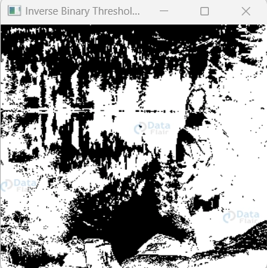
2. Inverse Binary Thresholding: cv2.THRESH_BINARY_INV

Similar to binary thresholding, the roles of black and white are reversed. Pixels with intensities greater than the threshold become black, while those below the threshold become white.

3. Truncated Thresholding: cv2.THRESH_TRUNC

In truncated thresholding, pixel values above the threshold are set to the threshold value itself. This creates a flat region at the threshold level.

4. Tozero Thresholding: cv2.THRESH_TOZERO

Here, pixel values below the threshold are set to zero, while those above the threshold remain unchanged.

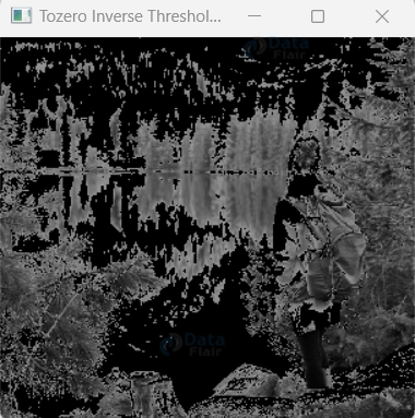
5. Tozero Inverse Thresholding: cv2.THRESH_TOZERO_INV

The opposite of tozero thresholding. Pixel values above the threshold are set to zero, and those below the threshold remain unchanged.

Syntax and Parameters:

The syntax for applying simple thresholding in OpenCV is as follows:

retval, threshold_output = cv2.threshold(input_image, threshold_value, max_value, threshold_type)

• Retval: The threshold value that was used. This may be important when using adaptive thresholding methods.
• Threshold_output: The output binary image after thresholding.
• Input_image: The input grayscale image on which thresholding is applied.
• Threshold_value: The threshold value to be used for comparison.
• Max_value: The maximum value assigned to pixels that satisfy the thresholding condition (usually 255 for white).
• Threshold_type: The type of thresholding method to be used (e.g., cv2.THRESH_BINARY, cv2.THRESH_BINARY_INV, etc.).

Code with Explanation:

Let’s illustrate simple thresholding using binary thresholding as an example:

import cv2
import numpy as np

# Read the grayscale image
image = cv2.imread(r"C:\Users\sanji\Desktop\DataFlair\Thresholding in Opencv\nature-img.jpg", cv2.IMREAD_GRAYSCALE)

# Threshold values
threshold_value = 150
max_value = 255



# Binary Thresholding
_, binary_threshold_output = cv2.threshold(image, threshold_value, max_value, cv2.THRESH_BINARY)

# Inverse Binary Thresholding
_, inverse_binary_threshold_output = cv2.threshold(image, threshold_value, max_value, cv2.THRESH_BINARY_INV)

# Truncated Thresholding
_, truncated_threshold_output = cv2.threshold(image, threshold_value, max_value, cv2.THRESH_TRUNC)

# Tozero Thresholding
_, tozero_threshold_output = cv2.threshold(image, threshold_value, max_value, cv2.THRESH_TOZERO)

# Tozero Inverse Thresholding
_, tozero_inverse_threshold_output = cv2.threshold(image, threshold_value, max_value, cv2.THRESH_TOZERO_INV)

# Create a window for each type of thresholding
cv2.namedWindow('Binary Thresholding', cv2.WINDOW_NORMAL)
cv2.namedWindow('Inverse Binary Thresholding', cv2.WINDOW_NORMAL)
cv2.namedWindow('Truncated Thresholding', cv2.WINDOW_NORMAL)
cv2.namedWindow('Tozero Thresholding', cv2.WINDOW_NORMAL)
cv2.namedWindow('Tozero Inverse Thresholding', cv2.WINDOW_NORMAL)

# Display the thresholded images
cv2.imshow('Binary Thresholding', binary_threshold_output)
cv2.imshow('Inverse Binary Thresholding', inverse_binary_threshold_output)
cv2.imshow('Truncated Thresholding', truncated_threshold_output)
cv2.imshow('Tozero Thresholding', tozero_threshold_output)
cv2.imshow('Tozero Inverse Thresholding', tozero_inverse_threshold_output)

cv2.waitKey(0)
cv2.destroyAllWindows()

Original Image :

Binary

Inverse Binary

Truncated

Tozero

Tozero inverse

In this code, we read a grayscale image and then apply all five types of simple thresholding using the cv2.threshold() function. We create a separate window for each thresholding output and display them using the cv2.imshow() function. The images will be displayed one after the other, and you can close the window by pressing any key.

Adaptive Thresholding in OpenCV: Mastering Image Segmentation with Dynamic Thresholds

In the ever-evolving world of image processing, adaptive thresholding stands as a versatile technique for tackling varying lighting conditions and image complexities. Unlike simple thresholding, where a fixed threshold is applied globally to the entire image, adaptive thresholding employs dynamic thresholds at each pixel’s local neighborhood. This adaptive nature empowers the algorithm to adapt to local changes, making it highly effective in scenarios with uneven illumination and varying contrasts.

Types of Adaptive Thresholding and Their Functions in OpenCV:

1. Adaptive Mean Thresholding: cv2.ADAPTIVE_THRESH_MEAN_C

Calculates the mean of the pixel intensities in a local neighborhood and uses it as the threshold value. Each pixel is compared to its local mean, which helps in handling varying illumination conditions.

2. Adaptive Gaussian Thresholding: cv2.ADAPTIVE_THRESH_GAUSSIAN_C

Identical to adaptive mean thresholding, but uses a Gaussian window to derive the threshold value based on the weighted sum of the pixel intensities in the immediate area rather than the mean.

Syntax and Parameters:

The syntax for applying adaptive thresholding in OpenCV is as follows:

threshold_output = cv2.adaptiveThreshold(input_image, max_value, adaptive_method, threshold_type, block_size, constant_value)

• Threshold_output: The output binary image after adaptive thresholding.
• Input_image: The input grayscale image on which adaptive thresholding is applied.
• Max_value: The maximum value assigned to pixels that satisfy the adaptive thresholding condition (usually 255 for white).
• Adaptive_method: The method used to calculate the adaptive threshold. It can be cv2.ADAPTIVE_THRESH_MEAN_C or cv2.ADAPTIVE_THRESH_GAUSSIAN_C.
• Threshold_type: The type of thresholding method to be used within the adaptive region (e.g., cv2.THRESH_BINARY, cv2.THRESH_BINARY_INV, etc.).
• Block_size: The size of the local neighborhood (should be an odd integer).
• constant_value: A constant value subtracted from the mean or weighted sum (only necessary for `cv2.ADAPTIVE_THRESH_MEAN_C`).

Code with Explanation:

import cv2

# Read the grayscale image
image = cv2.imread(r"C:\Users\sanji\Desktop\DataFlair\Thresholding in Opencv\nature-img.jpg", cv2.IMREAD_GRAYSCALE)

# Maximum pixel value for the thresholded image
max_value = 255

# Adaptive Mean Thresholding
block_size_mean = 11
constant_value_mean = 2
adaptive_mean_output = cv2.adaptiveThreshold(image, max_value, cv2.ADAPTIVE_THRESH_MEAN_C, cv2.THRESH_BINARY, block_size_mean, constant_value_mean)

# Adaptive Gaussian Thresholding
block_size_gaussian = 11
constant_value_gaussian = 2
adaptive_gaussian_output = cv2.adaptiveThreshold(image, max_value, cv2.ADAPTIVE_THRESH_GAUSSIAN_C, cv2.THRESH_BINARY, block_size_gaussian, constant_value_gaussian)

# Create windows for each type of adaptive thresholding
cv2.namedWindow('Adaptive Mean Thresholding', cv2.WINDOW_NORMAL)
cv2.namedWindow('Adaptive Gaussian Thresholding', cv2.WINDOW_NORMAL)

# Display the adaptive thresholded images
cv2.imshow('Adaptive Mean Thresholding', adaptive_mean_output)
cv2.imshow('Adaptive Gaussian Thresholding', adaptive_gaussian_output)

cv2.waitKey(0)
cv2.destroyAllWindows()

Original Image :

Adaptive Mean Thresholding :

Adaptive Gaussian Thresholding :

In this code, we read a grayscale image and then apply both types of adaptive thresholding using the cv2.adaptiveThreshold() function. We create separate windows for each adaptive thresholding output and display them using the cv2.imshow() function. The images will be displayed one after the other, and you can close the window by pressing any key.

Adding Borders in OpenCV: Amplifying Image Boundaries with copyMakeBorder() :

In the realm of image processing, adding borders to an image plays a crucial role in various applications. OpenCV offers a powerful function called copyMakeBorder(), which allows you to expand the image canvas and create a border of desired size and style. This function acts as a shield, safeguarding the image from unintended distortions and enhancing its visual appearance.

Syntax and Parameters:

The syntax for using copyMakeBorder() in OpenCV is as follows:

border_image = cv2.copyMakeBorder(src, top, bottom, left, right, border_type, value)

• Border_image: The output image with added borders.
• Src: The input image to which borders are added.
• top, bottom, left, right: The number of pixels to be added at the top, bottom, left, and right sides, respectively.
• Border_type: The type of border to be added. It can be one of the following:
• cv2.BORDER_CONSTANT: Adds a constant colored border. Use the value parameter to specify the color.
• cv2.BORDER_REPLICATE: Replicates the edge pixels to form a border.
• cv2.BORDER_REFLECT: Reflects the image content to form a border.
• cv2.BORDER_WRAP: Wraps the image content to form a border.
• cv2.BORDER_REFLECT_101: Reflects the image content with a slight adjustment to form a border.
• value: The colour value to be used when `cv2.BORDER_CONSTANT` is specified as the border type.

Code with Explanation :

Let’s demonstrate copyMakeBorder() by adding a red border to an image:

import cv2
import numpy as np

# Read the image
image = cv2.imread(r"C:\Users\sanji\Desktop\DataFlair\Thresholding in Opencv\nature-img.jpg")

# Define the border size in pixels
border_size = 20

# Define the border color (in BGR format)
border_color = (0, 0, 255)  # Red color

# Add the border using copyMakeBorder()
border_image = cv2.copyMakeBorder(image, border_size, border_size, border_size, border_size, cv2.BORDER_CONSTANT, value=border_color)

# Display the original image
cv2.imshow('Original Image', image)
cv2.waitKey(0)

# Display the bordered image
cv2.imshow('Bordered Image', border_image)
cv2.waitKey(0)

cv2.destroyAllWindows()

Original image :

Bordered Image :

In this code, we read an image and define the desired border size (in this case, 20 pixels). We chose the border color red (BGR value of `(0, 0, 255)`). The `copyMakeBorder()` function is then used to create a new image with a red border added to all four sides. We display the original and bordered images side by side for comparison.

Summary

In conclusion, we have traversed the captivating landscape of image processing, uncovering the secrets of thresholding and the art of adaptive techniques. From wielding the power of simple thresholding to embracing the dynamic nature of adaptive methods, we have witnessed how these tools can transform raw images into meaningful insights.

Through the magic of copyMakeBorder(), we have fortified our images with protective borders, elevating their aesthetics and safeguarding them against unwanted distortions. With newfound mastery over these techniques, we can now confidently embark on exciting computer vision endeavours, unlocking the potential to unravel complex visual challenges and unlock a world of possibilities.