Marshallian and Walrasian Approaches to Price Determination
Are you ready for UPSC Exam? Check your preparation with Free UPSC Mock Test
Price determination is a process of determining the cost of the goods sold and the services that are rendered to the market. It must be noted that the government of a country does not determine the price of the goods.
It is done by the two curves of demand and supply. The two approaches that have been in the notice are the Marshallian and the Walrasian approaches.

The Marshallian approach to Price Determination
Alfred Marshall was a British economist. The Marshallian era started in the late eighteen hundreds, with the publication of his book, named ‘ Principle of economics ‘.
However, before the introduction of the Marshallian approach to price determination, two more theories existed. One was the Jewel utility theory of pricing which worked on the principle that utility and price are directly proportional to each other.
The other approach was the Ricardian cost theory of pricing, which said price and cost are directly proportional to each other.
According to Marshal, in the case of perfect competition in an ideal market, the following should be done –
- The supply term shall be used in place of cost.
- The demand shall be used in place of utility.
He also says that the forces of both, demand and supply determined the equilibrium price. With this, he established the demand and supply theory of price determination.
He believes that the equilibrium price is neither solely determined by the demand factor (utility) nor by supply the factor(cost). The interaction between the two helps to determine the equilibrium price.
Otherwise, the demand might exceed supply, wherein the price will increase or the supply might exceed demand, wherein the price will fall.
Equilibrium is at the point of intersection of the demand curve (downward sloping) and the supply curve (upward sloping).
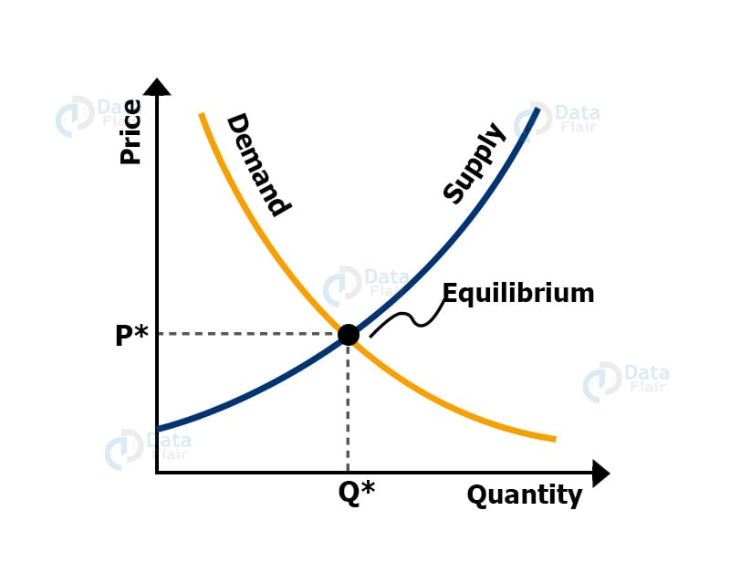
The following observations can be drawn from the above graph –
- The purple dot represents the point of intersection or the equilibrium.
- The red line represents the demand curve.
- The blue line represents the supply curve.
Marshall believed the supply curve to be of the three types, that is, downward sloping, horizontal, and upward sloping. This depends on the laws of the cost that are operating in the market, where the production is being done by the producer.
Types of Markets
The three types of markets are –
1. Market Period
It is also known as a very very short run. Herein, the supply of the commodity is constant and the demand is a variable, ie, it keeps on changing. The demand here is the determining factor, as it affects the price.
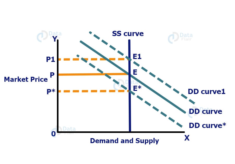
In the above diagram, the supply curve is a straight line because the supply is constant in the market period. The demand curve is downward sloping from left to right. The equilibrium is at the point where the supply and the demand curve intersect, that is, point E. The equilibrium price is OP.
However, if the demand increases, the supply being constant, the market price will increase from OP to OP1. If the demand decreases, keeping the supply constant, the price will fall from OP to OP*.
This brings us to conclude that demand and market prices are directly proportional to each other, the supply of the commodity being constant.
2. Normal Period
It can be further divided into a short-run and long-run normal period. In the short-run normal period, supply increases by a small amount. In a long-run normal period, supply increases by an adequate amount.
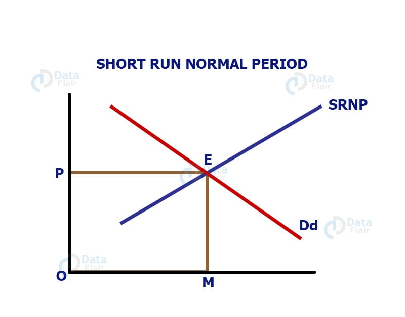
During the short run normal period, the price is equally determined by the demand and supply. Here demand and supply and price are equally directly proportional to each other. This means a rise in demand and supply will cause an increase in price.
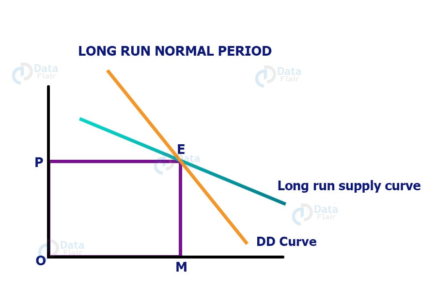
Herein, a rise in demand will lead to an increase in the supply of the commodity, but the price of the commodity will fall. This happens due to a lower marginal utility.
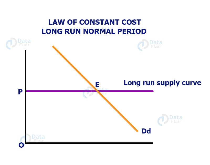
Here, if the demand increases, it leads to a rise in supply. However, in this case, the price remains constant. In this case, the marginal cost curve is horizontal.
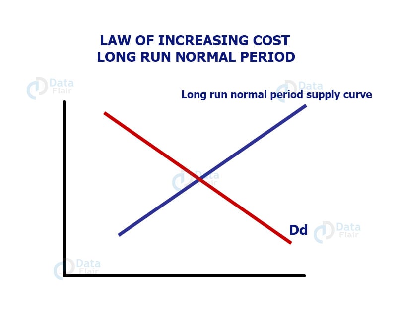
Here, an increase in demand will lead to an increase in price, which will further increase the price of the commodity.
If the market is experiencing a diminishing cost, the producer will increase the production, following which the price will decrease. In case of a constant cost, the supply line is horizontal
In the last three graphs, the supply curve, and marginal cost are alike.
It further concludes that price and supply may rise, however, in the long run, the supply will always rise, but the price may or may not rise.
3. Secular Period
It is also known as a very very long period, for say, over a century. This period helps in the historical analyses of the price trend. In this period, the price of the commodity might increase, remain the same, or decrease.
For example, the price of watches decreased over the years, the price of salt remained constant and the price of gold increased.
Walrasian Approach to Price Determination
Leon Walras was a French economist, whose book named ‘Elements of pure economics’ was published in the year 1889.
According to Walras, in real life, there is not one but several commodities. Therefore, we cannot get the equilibrium price for one commodity. He believes the economy has a general equilibrium. Under general equilibrium, we have demand and supply for not one but several commodities.
In the commodity market,
Dd (a) = fx ( Pa, Pb, Pc, Pd, …. Pn )
Ss (a) = fx (Pa, Pb, Pc, ….. Pn )
Wherein, P stands for price.
It believes that the price of a commodity is not solely dependent on the demand of that commodity but on the price of other commodities, too.
For example, the price of tea is not only dependent on the demand or supply of tea but on the price of sugar, sugarcane, milk, and more. Likewise, the supply of a good is not just related to the demand for that good but with other factors like storage, packing, transportation, and others.
In the factor market,
Dd (labour) =fx ( house rent, standard of living, environment, …. )
Ss (labour) = fx ( population, death rate, birth rate, wage rate …. )
Dd (capital) = fx ( interest rate, world market, the flow of foreign currency, … )
Ss (capital) = fx ( interest rate, globalization, free flow of capital, … )
Assumptions by Walras
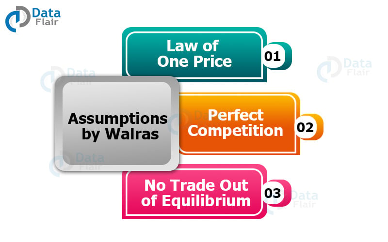
1. Law of one price
Any transaction that takes place in regard to the commodity, it should coincide with the price that has been already quoted at the instant.
2. Perfect Competition
In perfect competition, the traders behave in a competitive manner. Prices are taken as parameters to make optimized choices.
3. No trade out of equilibrium
A transaction related to the good should not take place outside the equilibrium.
Challenges faced by the Walrasian Model of Price Determination
Walras says that equilibrium price is neither uniqueness nor stability. However, it is a dynamic process, also known as the groping process or tatonnement process. It is the model for investigating the stability of equilibria.
But, even after several tries, he could not resolve some of the problems in the general equilibrium. Walras quoted, “in any pond there is water, but in the water, it is very difficult to find one stable level”.
He said, if all the markets are experiencing an equilibrium, then the one market that is not in equilibrium will itself find its equilibrium. His analysis was not accepted until modern times.
However, today the Nobel prize winner economists, Keneth Arrow, Lionel W McKenzie, Nicolas Bourbaki, and Gereard Debreu (1959) tried to solve the General equilibrium analysis.
Summary
We have seen Marshallian and Walrasian approaches to Price Determination. As discussed by Marshall, the price of single commodities in a very very short period market, wherein the supply is constant, the demand decides the price of the commodity.
In a long period, he said that the supply can adjust according to the demand in the market. He further also talked about the market price and normal price, wherein, the market price is the price that is prevailing in the market but the normal price is the average of the one-year market price.
An average of 1 year is the long run, an average of 4 months is short-run and the average of a hundred years is a very very long period. Due to his idea of the effect on the price of a commodity, keeping other factors constant, it was also called a Partial equilibrium approach to price determination.
However, Leon Walras believed that demand for a commodity is determined by not just by the price of that commodity. It is also affected by the price of other related and supplementary goods.
Where related goods are the goods that are used with each other and supplementary goods are the goods that are used in place of each other.
If you are Happy with DataFlair, do not forget to make us happy with your positive feedback on Google


Thank you for such detail……… I am really greatful to you.
It is so detailed and informational….looking for something like this, found it exactly here. Thank you so much.
awesome details
perfectly articulated in simple and precise manner i am very much grateful to you .
Begginers ke liye jaankari achhi hain