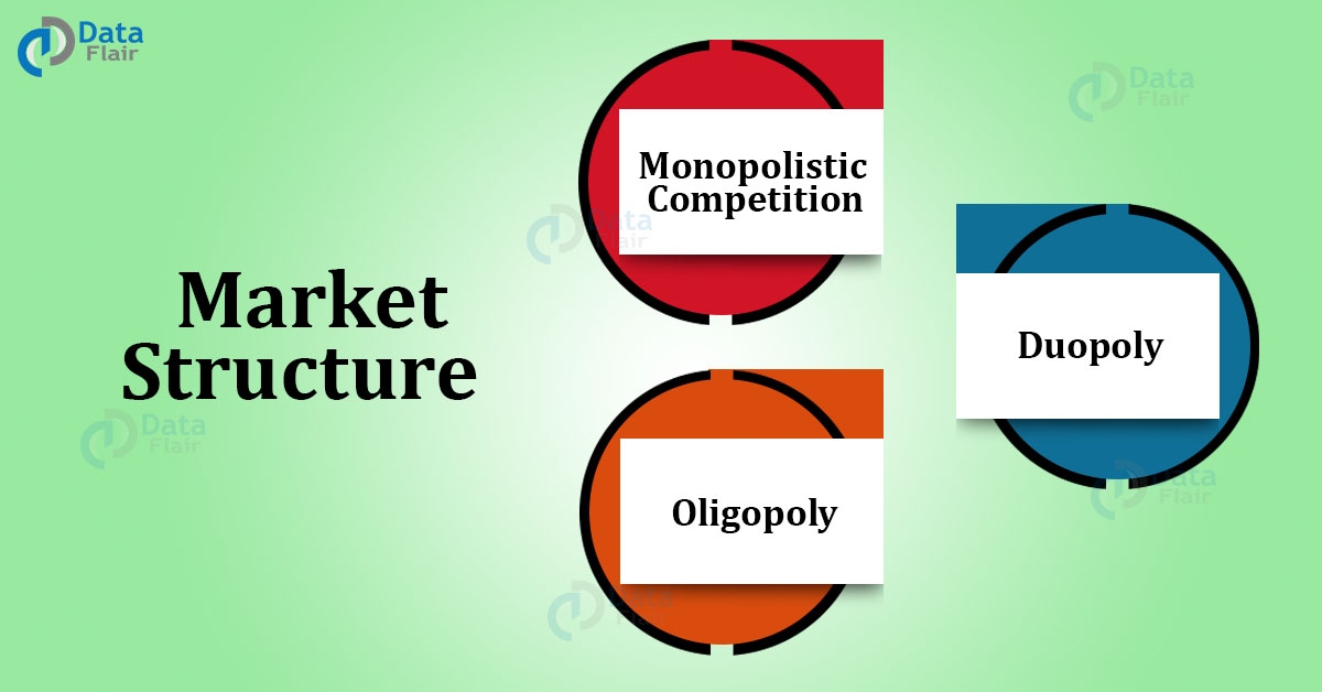
Market Structure: Monopolistic Competition, Duopoly, Oligopoly

Market morphology is the term that’s used for different types of markets. A monopoly market is where there are one seller and a large number of buyers.

A duopoly market is where there are two sellers and a large number of buyers are known as. An oligopoly market is where there are few sellers and a large number of buyers.

A bilateral monopoly is where there are a single buyer and one seller in the market. Let us learn more about the Market Structure.

Monopolistic Competition

A monopolist competition is a kind of imperfect competition wherein producers sell the products that are different from one another and therefore, are not perfect substitutes.

Chamberlin’s Model Assumptions

1. Product Differentiation and Non-price Competition

We get downward sloping curves with product differentiation. The products of different sellers are similar yet differentiated. To promote product differentiation, the firms incur considerable expenditure on advertising.

2. Myopia

The myopic vision of firms arises when the long run consists of identical short runs. Here, the decisions of one period do not impact the decisions of other periods.

3. Heroic Assumption (uniformity assumption)

Chamberlain assumes that both the demand and the cost curves for all differentiated are uniform throughout the group.

There is an interpretation that while each product is different, the consumer tastes for each are the same. It does not affect the price much.

Monopolistic Competition Vs. Oligopoly

In monopolistic competition, the firm’s actions wean the consumers from other firms.

However, the loss of the firm is so insignificant that it doesn’t notice or care to respond. This happens due to the close sustainability of the products.

In the case of an oligopoly market, the firms choose to respond to the changes that they observe in their consumers.

Product Differentiation and Demand Curve

Chamberlin suggested that it is not just the price and the quantity that affect the demand curve. It is also the product and the selling activities of the firm.

A change in the selling strategy of the firm, or consumer tastes, or products of other firms, can cause the demand curve to shift left or right.

Due to product differentiation, the producer gets some monopoly power. However, due to the close sustainability, there is limited power.

Industry and Product Group

A product group consists of products which are close and technical substitutes. This means they have high cross elasticities.

Due to the differentiation of the products, there will be no unique price in the group. But, this might cause a cluster of prices. However, this cluster changes as and when the demands and the costs change.

Long-Run Firm and Group Equilibrium under Monopolistic Competition

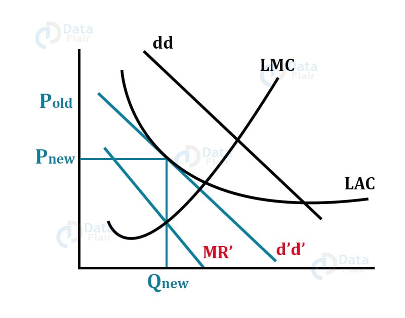
In the case of a short run, each firm behaves like a monopolist in its demand curve. However, it can’t stay there forever due to the supernatural π, new firms will enter. Though the new firms cannot produce the same product but can get somewhat close to it.

Due to this, the firm’s demand curve will shift to the left from dd to d’d’. The final equilibrium will be tangent to the LAC Curve and the firm will operate at less than full capacity. The tangency to the LAC Curve ensures no supernatural profits remain.

Even in the long-run, the firm can only make normal profits. Its price is higher and the output is lower as compared to PC. This shows that the existence of supernatural profits is not an indicator of monopoly power.

Another significant implication is that as more and more firms enter, the LR in the demand curve of the firm keeps on becoming flattered. This happens because the firm is earning supernormal profit and the new firm will try to produce a closer substitute to it.

The new firms that enter the group will occupy positions between the old demand curves.

Economic Efficiency under Monopolistic Competition

In the model, the firm never touches the minimum LAC. the amount by which the LR output falls short of the socially ideal output. That is why there is excess capacity.

One of the reasons for this action is the downward sloping demand curve. Another reason could be the entry of large firms in the market. The markets get split among the great number of firms and excess capacity results.

It is also believed that in the monopolistic competition, the firms spend on advertising and other selling costs.

Chamberlin argues that the social cost of producing the social cost of providing differentiated goods to consumers. Therefore, it is not the real excess capacity.

The real excess capacity will be when the firms abandon the price competition and begin to compete on the non-price terms and more differentiation. In the case price competition is absent, the demand curve is irrelevant.

However, Kaldor argues that the presence of the institutional monopolies might break the excess capacity theory of Chamberlin. Institutional monopoly may be a cost advantage. That is something that can give supernatural profits. Thus, it can reduce excess capacity.

Adding to this, Kaldor said that one can also reduce excess capacity. But switching production also has some costs.

Duopoly Model

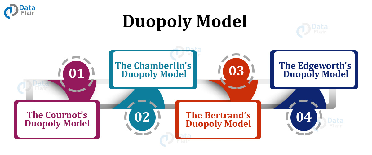
There is not one but several economists who worked on the Duopoly Model. Some of them are –

1. The Cournot’s Duopoly Model
2. The Chamberlin’s Duopoly Model
3. The Bertrand’s Duopoly Model
4. The Edgeworth’s Duopoly Model

1. Cournot’s Duopoly Model

Augustin Cournot was a French economist. He was the first one to develop a formal duopoly model in the year 1838.

Assumptions of the Cournot Model

• Two firms, each owing artesian mineral water well.
• Both operate the wells at zero marginal cost.
• They face a demand curve with a constant negative slope.
• The competitor will not react to his decision of changing his price. This is also known as the behavioral assumption.

Diagrammatic Representation

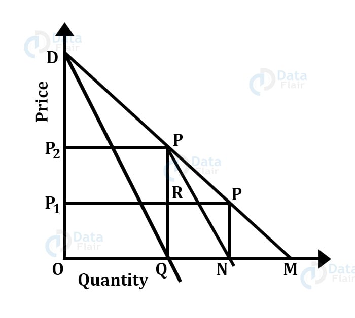
To start, suppose that there are only two firms, named, A and B. A is the only seller of the mineral water in the market. To maximize his profits or revenue, he sells the quantity OQ. Here, MC = 0 MR, the price at OP2. The total profit is OP2PQ.

Now, when B enters the market and the market that is open to him is QM. QM is half of the total market. B assumes that A will not change his price and output since he is already making the maximum profit.

To get maximum revenue, B sells ON at price OP1. with this, his total revenue is maximum at QRP’N.

With the entry of B, the price falls to Op1. The expected profit of A falls OP1PQ. This induces A to adjust its price and output according to the changing conditions. Assuming that B will not change his output and price since he is making maximum profit.

This is now B’s turn to react and the same thing will repeat as above.

In the successive periods, this process of action and reaction continues. In such a way, A continues to lose its market share and B continues to gain. The final result is when both of their market shares are at one third.

We can stretch the Cournot’s model of duopoly to the general oligopoly. For instance, if there are three sellers, the industry and the firm will be in equilibrium when each firm supplies 1/3rd of the market.

Thus, three sellers together, supply 3/4th of the share of the market. And the 1/4th share remains unsupplied.

The formula that determines the share of each seller in an oligopolistic market is –
Q-f- (n+1) , where Q = market size and n = number of sellers.

Cournot concluded that each seller ultimately supplies one-third of the market. Here, it charges the same price. This happens while one-third of the market is still unsupplied.

Criticism of Cournot’s Model

Although his model yields a stable equilibrium, the Cournot’s model is criticized on the following grounds –

The behavioral assumption is naive to the extent that it implies that firms continue to make wrong calculations about the competitor’s behavior. Each seller assumes that his rival will not change his price or output even though he continues to observe the opposite.

The unrealistic assumption of the zero cost of production. In case, this assumption is not taken, it will not alter his position.

2. Chembelrin’s Duopoly Model

This model recognizes the interdependence of the firms in the market. He argues that in the real world of oligopoly firms, the firms will not learn from their past experiences. Chamberlain makes the same assumptions as of the exponents of the old classical model.

Chamberlain’s model is also based on the assumption of equal size with identical costs.

However, his recognition of the interdependence of the firms in the oligopolistic market gave a result that was quite different from that of Cournot. Chamberlain argues that the firms are aware of the fact that their output or price will surely invite reactions from other firms.

Therefore, the price-war is not visualized in the oligopolistic markets. With this, he also rules out the possibility of the firms adjusting their outputs over some time. Therefore, reaching an equilibrium, at an output level lower than that would be reached under monopoly.

According to him, recognition of possible sharp reactions to an oligopolistic firm’s price or the output manipulations will avoid harmful competition amongst the firms in such a market. This would result in a stable industry equilibrium with monopoly price and output.

He further believed that no collision is required to obtain this solution.

In the case of farms in an oligopolistic market are aware of their mutual dependence and willing to learn from their past experiences. To maximize their individual and joint profits, they will charge the monopoly price.

The Chamberlin Model

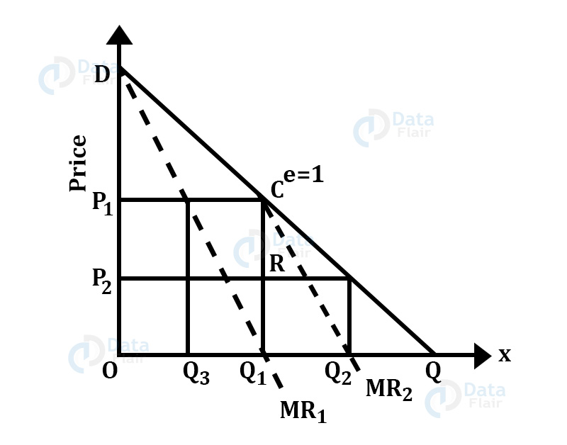
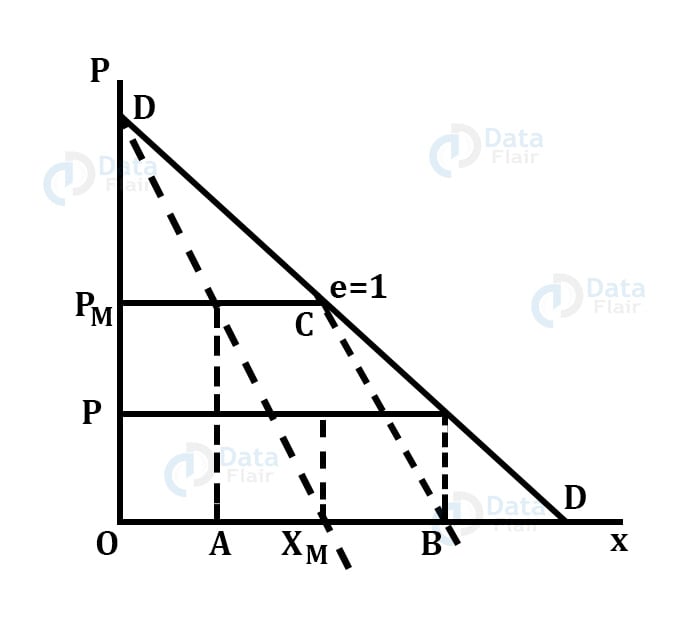
Chamberlain’s model is explained in the framework of a duopoly market. Like Cournot, Chamberlain assumes linear demand for the product. For simplicity, an assumption is made that even in this case, the cost of producing the goods is zero.

In the above figure, DQ is the market demand curve. If firm A enters the market, it will produce output OQ1 because, at this level of output, the marginal revenue is equal to marginal cost. The firm might charge OP1, which is the monopoly price.

This will lead to the maximization of profits. At price OP, the elasticity of demand is unitary.

If firm B enters the market at this stage, it considers its demand curve is CQ. It will produce Q1Q2 to maximize its profits. It will move to the price OP2.

After realizing that it can no longer sell at QQ1 quantity, it decides to reduce the output to QQ3. Firm B continues to produce Q1Q2 quantity which is the same as Q3Q1. The industry output is OQ1and the price rises to OP1. Both the firms, A and B consider it an ideal situation.

The joint output of both firms is monopoly output and they charge a monopoly price. Thus, considering this assumption, the market will be shared equally between the two firms.

Appraisal of the Model

Chamberlin’s model is certainly more realistic than the other models. It assumes that the firms recognize the interdependence and then act in a manner that the monopoly solution is reached. In the real world of oligopoly, certain difficulties are faced in reaching this solution.

In the absence of collusion, the firms should have a good knowledge of the market demand curve which is almost impossible to reach.

Furthermore, he also ignores entry. In real practice, the oligopolistic markets are rarely closed. So, if we consider entry, it would not be certain that the stable monopoly solution will ever be reached.

3. Bertrand’s Duopoly Model

Bertrand was a French Mathematician who developed his model of the duopoly in 1883. His model is different from that of Cournot in respect to its behavioral assumption.

Under Bertrand’s model, each seller determines his price on the assumption that his rival’s price and not output remains constant.

Bertrand’s model focuses on price competition. His analytical tools are the reaction function of the duopolists. The reaction functions are derived based on the iso-profit curves.

He assumed that there were only two firms, ie, A and B. The prices are measured along the horizontal and vertical axes.

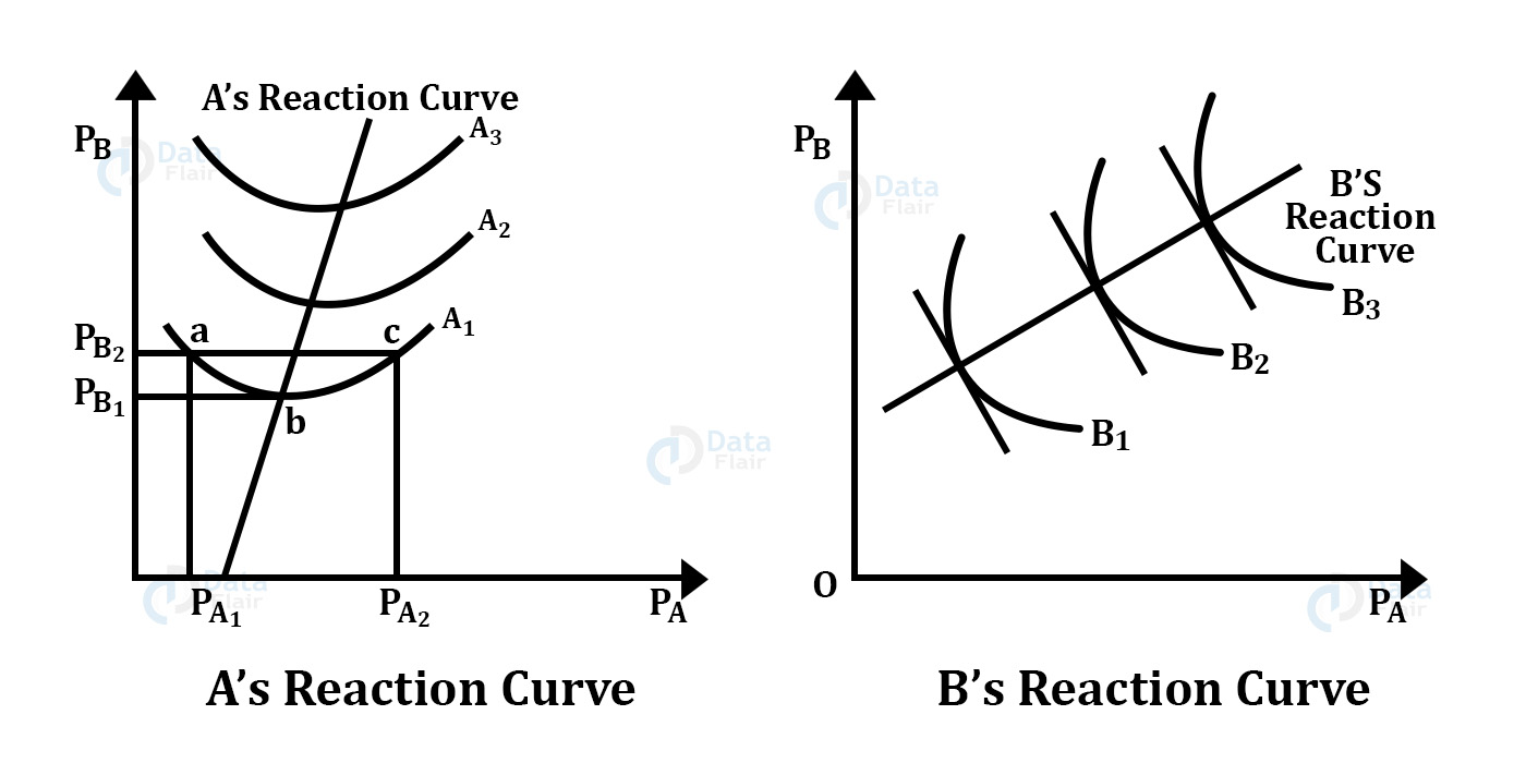
The iso-profit curves are drawn based on the prices of the two firms. The iso-profit curves of firm A are convex to its price axis and the curves of firm B are convex to PB.

When the firm B reduces its price, A can either increase or reduce it. Firm A will reduce its price when he is at point c. It will raise its price when he is at point A. However, there is no limit to which the price adjustment is possible.

The same applies to all other iso-profit curves. The equilibrium of the duopolists suggested by Bertrand’s Model may be obtained by putting together the reaction curves of firm A and firm B.

Criticism of the Model

This model was criticized because it is the same as Cournot’s model. Bertrand’s implicit behavioral assumption that the firms don’t learn from their past experiences seems to be unrealistic.

If the cost is assumed 0, the price will fluctuate between zero and the upper limit of price. It will not stabilize at a point.

4. Edgeworth’s Duopoly Model

Edgeworth’s Duopoly Model came up in 1897. He follows Bertrans’s assumption that each seller assumes his rival’s price instead of his output, to remain constant.

Representation of Edgeworth’s Model of Duopoly

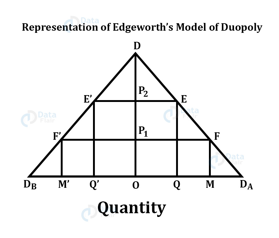
In the figure, we have to assume that there are two sellers. These firms, A and B face identical demand curves. A’s demand curve is DDB. Seller A has the maximum capacity of output OM and B has the maximum output capacity of OM’. ODA measures the price.

To commence with, let us assume that A is the only seller in the market. He sells OQ and charges OP2.

The monopoly cost under zero cost is equal to OP2EQ. Now if B enters the market, he assumes that A will not change his price since he is making maximum profit. Firm B sets its price slightly below A’s price and can sell his total output. Seller A, on the other hand, has his sales gone down.

To regain his market, A sets his price slightly below the price of B. This creates a price-war between the sellers.

The price-war takes the form of price-cutting which continues until price reaches OP1. At this level both the firms, A and B can sell their entire output- A sells OQ and B sells OQ. The price of OP1 can be stable. However. According to Edgeworth, price OP1 should not be stable.

In all, Edgeworth’s model is based on a naive assumption that a rival will never change his price even after being proved repeatedly wrong. However, Edgeworth’s model is an improved version of Cournot’s model.

Oligopoly Market

An Oligopoly market is the kind of market where the industry is dominated by a small group of large sellers. It reduced the competition in the market, as it can lead to various forms of collisions.

Chamberlain’s Oligopoly Model

Chamberlin said that if the firms do not recognize their interdependence, the industry will reach either of the Cournot’s equilibrium. He says that each form acts independently on the assump­tion that the rivals will either keep their output constant.

The industry will reach the Bertrand equilibrium, trying to maximize its profit on the assumption that the other rivals will not change their price.

However, he rejected the assumption of the independent actions by the competitors. He believes that firms are not as naive as assumed by Cournot and Bertrand.

His model can be best understood in a duopoly market.

It is vital to know that Chamberlin’s model of Oligopoly observed a kinked demand curve.

Chamberlin’s model is a bit more advanced over the previous models. As it assumes that the firms are sophisticated enough to realize their interdependence. Also, further, it leads to a stable equilibrium, which is the monopoly solution. He model is also known as a ‘closed’ model.

If the entry does occur it is uncertain that a stable monopoly solution will ever be reached. This will be unless there are special assumptions regarding the behavior of the old firms and the new entrants.

Summary

This article talked about the various forms of market structures that exist in the market. The types of markets are monopoly, duopoly, and oligopoly. Different structures of markets have their pros and cons and affect the market conditions accordingly.

In a monopoly market, there exists one seller and multiple numbers of buyers. In a duopolistic market, there exist two sellers and multiple numbers of buyers. In the case of an oligopolistic market, there are some sellers and several buyers.