Data Mining Algorithms – 13 Algorithms Used in Data Mining

In our last tutorial, we studied  Data Mining Techniques. Today,  we will learn Data Mining Algorithms.

We will cover all types of Algorithms in Data Mining: Statistical Procedure Based Approach, Machine Learning-Based Approach, Neural Network, Classification Algorithms in Data Mining, ID3 Algorithm, C4.5 Algorithm, K Nearest Neighbors Algorithm, Naïve Bayes Algorithm, SVM Algorithm, ANN Algorithm, 48 Decision Trees, Support Vector Machines, and SenseClusters.

So, let’s start Data Mining Algorithms.

What are Data Mining Algorithms?

There are too many Data Mining Algorithms present. We will discuss each of them one by one.

• These are the examples, where the data analysis task is Classification Algorithms in Data Mining-

• A bank loan officer wants to analyze the data in order to know which customer is risky or which are safe.

• A marketing manager at a company needs to analyze a customer with a given profile, who will buy a new computer.

Why Algorithms Used In Data Mining?

Here, are some reason which gives the answer of usage of Data Mining Algorithms:

• In today’s world of “big data”, a large database is becoming a norm. Just imagine there present a database with many terabytes.

• As Facebook alone crunches 600 terabytes of new data every single day. Also, the primary challenge of big data is how to make sense of it.

• Moreover, the sheer volume is not the only problem. Also, big data need to diverse, unstructure and fast changing. Consider audio and video data, social media posts, 3D data or geospatial data. This kind of data is not easily categorized or organized.

• Further, to meet this challenge, a range of automatic methods for extracting information.

Types of Algorithms In Data Mining

Here, 13 Data Mining Algorithms are discussed-

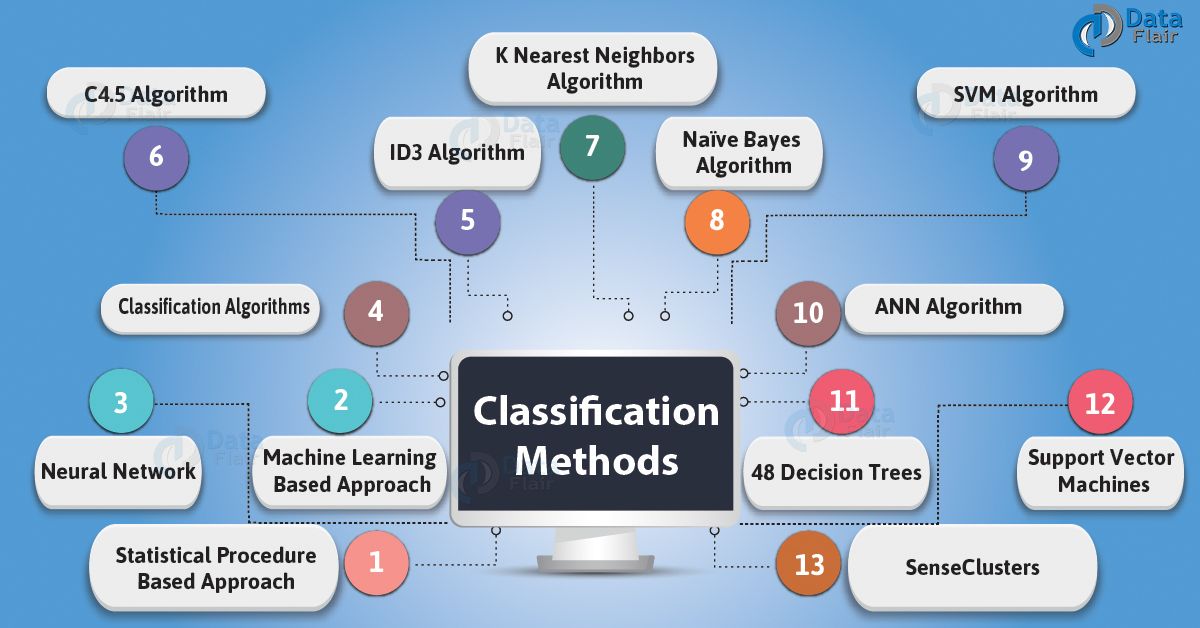
Data Mining Algorithms – Types

a. Statistical Procedure Based Approach

There are two main phases present to work on classification. That can easily identify the statistical community.

The second, “modern” phase concentrated on more flexible classes of models. In which many of which attempt has to take. That provides an estimate of the joint distribution of the feature within each class. That can, in turn, provide a classification rule.

Generally, statistical procedures have to characterize by having a precise fundamental probability model. That used to provides a probability of being in each class instead of just a classification. Also, we can assume that techniques will use by statisticians.

Hence some human involvement has to assume with regard to variable selection. Also, transformation and overall structuring of the problem.

b. Machine Learning-Based Approach

Generally, it covers automatic computing procedures. That was based on logical or binary operations. That use to learn a task from a series of examples.

Here, we have to focus on decision-tree approaches. As classification results come from a sequence of logical steps. These classification results are capable of representing the most complex problem given. Such as genetic algorithms and inductive logic procedures (I.LP.) are currently under active improvement.

Also, its principle would allow us to deal with more general types of data including cases. In which the number and type of attributes may vary.

This approach aims to generate classifying expressions. That is simple enough to understand by the human. And must mimic human reasoning to provide insight into the decision process.

Like statistical approaches, background knowledge may use in development. But the operation is assumed without human interference.

c. Neural Network

The field of Neural Networks has arisen from diverse sources. That is ranging from understanding and emulating the human brain to broader issues. That is of copying human abilities such as speech and use in various fields. Such as banking, in classification program to categorize data as intrusive or normal.

Generally, neural networks consist of layers of interconnected nodes. That each node producing a non-linear function of its input. And input to a node may come from other nodes or directly from the input data. Also, some nodes are identified with the output of the network.

On the basis of this, there are different applications for neural networks present. That involve recognizing patterns and making simple decisions about them.

In airplanes, we can use a neural network as a basic autopilot. In which input units read signals from the various instruments and output units. That modifying the plane’s controls appropriately to keep it safely on course. Inside a factory, we can use a neural network for quality control.

d. Classification Algorithms in Data Mining

It is one of the Data Mining. That is used to analyze a given data set and takes each instance of it. It assigns this instance to a particular class. Such that classification error will be least. It is used to extract models. That define important data classes within the given data set. Classification is a two-step process.

During the first step, the model is created by applying a classification algorithm. That is on training data set.

Then in the second step, the extracted model is tested against a predefined test data set. That is to measure the model trained performance and accuracy. So classification is the process to assign class label from a data set whose class label is unknown.

e. ID3 Algorithm

This Data Mining Algorithms starts with the original set as the root hub. On every cycle, it emphasizes through every unused attribute of the set and figures. That the entropy of attribute. At that point chooses the attribute. That has the smallest entropy value.

The set is S then split by the selected attribute to produce subsets of the information.

This Data Mining algorithms proceed to recurse on each item in a subset. Also, considering only items never selected before. Recursion on a subset may bring to a halt in one of these cases:

• Every element in the subset belongs to the same class (+ or -), then the node is turned into a leaf and

• labeled with the class of the examples

• If there are no more attributes to select but the examples still do not belong to the same class. Then the node is turned into a leaf and labeled with the most common class of the examples in that subset.

• If there are no examples in the subset, then this happens. Whenever parent set found to be matching a specific value of the selected attribute.

• For example, if there was no example matching with marks >=100. Then a leaf is created and is labeled with the most common class of the examples in the parent set.

Working steps of Data Mining Algorithms is as follows,

• Calculate the entropy for each attribute using the data set S.

• Split the set S into subsets using the attribute for which entropy is minimum.

• Construct a decision tree node containing that attribute in a dataset.

• Recurse on each member of subsets using remaining attributes.

f. C4.5 Algorithm

C4.5 is one of the most important Data Mining algorithms, used to produce a decision tree which is an expansion of prior ID3 calculation. It enhances the ID3 algorithm. That is by managing both continuous and discrete properties, missing values. The decision trees created by C4.5. that use for grouping and often referred to as a statistical classifier.

C4.5 creates decision trees from a set of training data same way as an Id3 algorithm. As it is a supervised learning algorithm it requires a set of training examples. That can see as a pair: input object and the desired output value (class).

The algorithm analyzes the training set and builds a classifier. That must have the capacity to accurately arrange both training and test cases.

A test example is an input object and the algorithm must predict an output value. Consider the sample training data set S=S1, S2,…Sn which is already classified.

Each sample Si consists of feature vector (x1,i, x2,i, …, xn,i). Where xj represent attributes or features of the sample. The class in which Si falls. At each node of the tree, C4.5 selects one attribute of the data. That most efficiently splits its set of samples into subsets such that it results in one class or the other.

The splitting condition is the normalized information gain. That is a non-symmetric measure of the difference. The attribute with the highest information gain is chosen to make the decision. General working steps of algorithm is as follows,

Assume all the samples in the list belong to the same class. If it is true, it simply creates a leaf node for the decision tree so that particular class will select.

None of the features provide any information gain. If it is true, C4.5 creates a decision node higher up the tree using the expected value of the class.

An instance of previously-unseen class encountered. Then, C4.5 creates a decision node higher up the tree using the expected value.

g. K Nearest Neighbors Algorithm

The closest neighbor rule distinguishes the classification of an unknown data point. That is on the basis of its closest neighbor whose class is already known.

M. Cover and P. E. Hart purpose k nearest neighbor (KNN). In which nearest neighbor is computed on the basis of estimation of k. That indicates how many nearest neighbors are to consider to characterize.

It makes use of the more than one closest neighbor to determine the class. In which the given data point belongs to and so it is called as KNN. These data samples are needed to be in the memory at the runtime.
Hence they are referred to as memory-based technique.

Bailey and A. K. Jain enhances KNN which is focused on weights. The training points are assigned weights. According to their distances from sample data point. But at the same, computational complexity and memory requirements remain the primary concern.

To overcome memory limitation size of data set is reduced. For this, the repeated patterns. That don’t include additional data are also eliminated from training data set.

To further enhance the information focuses which don’t influence the result. That are additionally eliminated from training data set.

The NN training data set can organize utilizing different systems. That is to enhance over memory limit of KNN. The KNN implementation can do using ball tree, k-d tree, and orthogonal search tree.

The tree-structured training data is further divided into nodes and techniques. Such as NFL and tunable metric divide the training data set according to planes. Using these algorithms we can expand the speed of basic KNN algorithm. Consider that an object is sampled with a set of different attributes.

Assuming its group can determine from its attributes. Also, different algorithms can use to automate the classification process. In pseudo code, k-nearest neighbor algorithm can express,

K ← number of nearest neighbors

For each object Xin the test set do

calculate the distance D(X,Y) between X and every object Y in the training set

neighborhood ← the k neighbors in the training set closest to X

X.class ← SelectClass (neighborhood)

End for

h. Naïve Bayes Algorithm

The Naive Bayes Classifier technique is based on the Bayesian theorem. It is particularly used when the dimensionality of the inputs is high.

The Bayesian Classifier is capable of calculating the possible output. That is based on the input. It is also possible to add new raw data at runtime and have a better probabilistic classifier.

This classifier considers the presence of a particular feature of a class. That is unrelated to the presence of any other feature when the class variable is given.

For example, a fruit may consider to be an apple if it is red, round.

Even if these features depend on each other features of a class. A naive Bayes classifier considers all these properties to contribute to the probability. That it shows this fruit is an apple. Algorithm works as follows,

Bayes theorem provides a way of calculating the posterior probability, P(c|x), from P(c), P(x), and P(x|c). Naive Bayes classifier considers the effect of the value of a predictor (x) on a given class (c). That is independent of the values of other predictors.

P(c|x) is the posterior probability of class (target) given predictor (attribute) of class.

P(c) is called the prior probability of class.

P(x|c) is the likelihood which is the probability of predictor of given class.

P(x) is the prior probability of predictor of class.

i. SVM Algorithm

SVM has attracted a great deal of attention in the last decade. It also applied to various domains of applications. SVMs are used for learning classification, regression or ranking function.

SVM is based on statistical learning theory and structural risk minimization principle. And have the aim of determining the location of decision boundaries. It is also known as a hyperplane. That produces the optimal separation of classes. Thereby creating the largest possible distance between the separating hyperplane.

Further, the instances on either side of it have been proven. That is to reduce an upper bound on the expected generalization error.

The efficiency of SVM based does not depend on the dimension of classified entities. Though, SVM is the most robust and accurate classification technique. Also, there are several problems.

The data analysis in SVM is based on convex quadratic programming. Also, expensive, as solving quadratic programming methods. That need large matrix operations as well as time-consuming numerical computations.

Training time for SVM scales in the number of examples. So researchers strive all the time for more efficient training algorithm. That resulting in several variant based algorithm.

SVM can also extend to learn non-linear decision functions. That is by first projecting the input data onto a high-dimensional feature space. As by using kernel functions and formulating a linear classification problem. The resulting feature space is much larger than the size of a dataset. That is not possible to store on popular computers.

Investigation of this issues leads to several decomposition based algorithms. The basic idea of decomposition method is to split the variables into two parts:

a set of free variables called as a working set. That can update in each iteration and set of fixed variables. That are fix during a particular. Now, this procedure have to repeat until the termination conditions are met

The SVM was developed for binary classification. And it is not simple to extend it for multi-class classification problem. The basic idea to apply multi-classification to SVM. That is to decompose the multi-class problems into several two-class problems. That can address using several SVMs.

J. ANN Algorithm

This is the types of computer architecture inspire by biological neural networks. They are used to approximate functions. That can depend on a large number of inputs and are generally unknown.

They are presented as systems of interconnected “neurons”. That can compute values from inputs. Also, they are capable of machine learning as well as pattern recognition. Due to their adaptive nature.

An artificial neural network operates by creating connections between many different processing elements. That each corresponding to a single neuron in a biological brain. These neurons may actually construct or simulate by a digital computer system.

Each neuron takes many input signals. Then based on an internal weighting. That produces a single output signal that is sent as input to another neuron.

The neurons are interconnected and organized into different layers. The input layer receives the input and the output layer produces the final output.

In general, one or more hidden layers are sandwiched between the two. This structure makes it impossible to forecast or know the exact flow of data.

Artificial neural networks start out with randomized weights for all their neurons. This means that they need to train to solve the particular problem for which they are proposed. A back-propagation ANN is trained by humans to perform specific tasks.

During the training period, we can test whether the ANN’s output is correct by observing a pattern. If it’s correct the neural weightings produce that output is reinforced. if the output is incorrect, those weightings responsible diminish.

Implemented on a single computer, a network is slower than more traditional solutions. The ANN’s parallel nature allows it to built using many processors. That gives a great speed advantage at very little development cost.

The parallel architecture allows ANNs to process amounts of data very in less time. It deals with large continuous streams of information. Such as speech recognition or machine sensor data. ANNs can operate faster as compared to other algorithms.

An artificial neural network is useful in a variety of real-world applications. Such as visual pattern recognition and speech recognition. That deals with complex often incomplete data.

Also, recent programs for text-to-speech have utilized ANNs. Many handwriting analysis programs are currently using ANNs.

K. 48 Decision Trees

A decision tree is a predictive machine-learning model. That decides the target value of a new sample. That based on various attribute values of the available data. The internal nodes of a decision tree denote the different attributes.

Also, the branches between the nodes tell us the possible values. That these attributes can have in the observed samples. While the terminal nodes tell us the final value of the dependent variable.

The attribute is to predict is known as the dependent variable. Since its value depends upon, the values of all the other attributes. The other attributes, which help in predicting the value of the dependent variable. That are the independent variables in the dataset.

The J48 Decision tree classifier follows the following simple algorithm. To classify a new item, it first needs to create a decision tree. That based on the attribute values of the available training data.

So, whenever it encounters a set of items. Then it identifies the attribute that discriminates the various instances most clearly.

This feature is able to tell us most about the data instances. So that we can classify them the best is said to have the highest information gain.

Now, among the possible values of this feature. If there is any value for which there is no ambiguity. That is, for which the data instances falling within its category. It has the same value for the target variable. Then we stop that branch and assign to it the target value that we have obtained.

For other cases, we look for another attribute that gives us the highest information gain. We continue to get a clear decision. That of what combination of attributes gives us a particular target value.

In the event that we run out of attributes. If we cannot get an unambiguous result from the available information. We assign this branch a target value that the majority of the items under this branch own.

Now that we have the decision tree, we follow the order of attribute selection as we have obtained for the tree. By checking all the respective attributes. And their values with those seen in the decision tree model. we can assign or predict the target value of this new instance.

The above description will be more clear and easier to understand with the help of an example. Hence, let us see an example of J48 decision tree classification.

l. Support Vector Machines

Support Vector Machines are supervised learning methods. That used for classification, as well as regression. The advantage of this is that they can make use of certain kernels to transform the problem. Such that we can apply linear classification techniques to non-linear data.

Applying the kernel equations. That arranges the data instances in a way within the multi-dimensional space. That there is a hyperplane that separates data instances of one kind from those of another.

The kernel equations may be any function. That transforms the non-separable data in one domain into another domain. In which the instances become separable. Kernel equations may be linear, quadratic, Gaussian, or anything else. That achieves this particular purpose.

Once we manage to divide the data into two distinct categories, our aim is to get the best hyperplane. That is to separate the two types of instances. This hyperplane is important, it decides the target variable value for future predictions. We should decide upon a hyperplane that maximizes the margin. That is between the support vectors on either side of the plane.

Support vectors are those instances that are either on the separating planes. The explanatory diagrams that follow will make these ideas a little more clear.

In Support Vector Machines the data need to be separate to be binary. Even if the data is not binary, these machines handle it as though it is. Further completes the analysis through a series of binary assessments on the data.

M. SenseClusters (an adaptation of the K-means clustering algorithm)

We have made use of SenseClusters to classify the email messages. SenseCluster available package of Perl programs. As it was developed at the University of Minnesota Duluth. That we use for automatic text and document classification. The advantage of SenseClusters is that it does not need any training data;

It makes use of unsupervised learning methods to classify the available data.

Now, particularly in this section will understand the K-means clustering algorithm. That has been used in SenseClusters. Clustering is the process in which we divide the available data. That instances of a given number of sub-groups. These sub-groups are clusters, and hence the name “Clustering”.

To put it, the K-means algorithm outlines a method. That is to cluster a particular set of instances into K different clusters. Where K is a positive integer. It should notice K-means clustering algorithm requires a number of clusters from the user. It cannot identify the number of clusters by itself.

However, SenseClusters has the facility of identifying the number of clusters. That the data may comprise of.

The K-means clustering algorithm starts by placing K centroids. Then each of the available data instances has to assign a particular centroid. That depends on a metric like Euclidian distance, Manhattan distance, Minkowski distance, etc.

The position of the centroid has to recalculate every time an instance is added to the cluster. This continues until all the instances are group into the final required clusters.

Since recalculating the cluster centroids may alter the cluster membership. Also, cluster memberships are also verified once the position of the centroid changes.

This process continues till there is no further change in the cluster membership. And there is as little change in the positions of the centroids as possible.

The initial position of the centroids is thus very important. Since this position affects all the future steps in the K-means clustering algorithm. Hence, it is always advisable to keep the cluster centers as far away from each other as possible.

If there are too many clusters, then clusters resemble each other. And they are in the vicinity of each other that need to be club together.

Moreover, if there are few clusters then clusters that are too big. And may contain two or more sub-groups of different data instances that must be a divide.

The K-means clustering algorithm is thus a simple to understand. Also, a method by which we can divide the available data into sub-categories.

So, this was all about Data Mining Algorithms. Hope you like our explanation.

Conclusion

As a result, we have studied Data Mining Algorithms. Also, we have learned each type of Data Mining algorithm.  Furthermore, if you feel any query, feel free to ask in a comment section.