Earthquake Prediction using Machine Learning

With this Machine Learning Project, we will build an earthquake predictor using machine learning algorithms. For this project, we will use a Random forest Classifier, Support Vector Classifier, and Gradient Boosting Algorithm to predict.

So, let’s build this system.

Earthquake Prediction System

Earthquakes were once thought to result from supernatural forces in the prehistoric era. Aristotle was the first to identify earthquakes as a natural occurrence and to provide some potential explanations for them in a truly scientific manner. One of nature’s most destructive dangers is earthquakes. Strong earthquakes frequently have negative effects.

A lot of devastating earthquakes occasionally occur in nations like Japan, the USA, China, and nations in the middle and far east. Several major and medium-sized earthquakes have also occurred in India, which have resulted in significant property damage and fatalities. One of the most catastrophic earthquakes ever recorded occurred in Maharastra early on September 30, 1993. One of the main goals of researchers studying earthquake seismology is to develop effective predicting methods for the occurrence of the next severe earthquake event that may allow us to reduce the death toll and property damage.

Most earthquakes, or 90%, are natural and result from tectonic activity. 10% of the remaining characteristics are associated with volcanism, man-made consequences, or other variables. Natural earthquakes are those that occur naturally and are typically far more powerful than other kinds of earthquakes. The continental drift theory and the plate-tectonic theory are the two hypotheses that deal with earthquakes.

Random Forest

It is a type of machine learning algorithm that is very famous nowadays. It generates a random decision tree and combines it into a single forest. It features a decision model to increase accuracy. These trees divide the predictor space using a series of binary splits (“splits”) on distinct variables. The tree’s “root” node represents the entire predictor space. The final division of the predictor space is made up of the “terminal nodes,” which are nodes that are not split. Depending on the value of one of the predictor variables, each nonterminal node divides into two descendant nodes, one on the left and one on the right. If a continuous predictor variable is smaller than a split point, the points to the left will be the smaller predictor points, and the points to the right will be the larger predictor points. The values of a categorical predictor variable Xi come from a small number of categories. To divide a node into its two descendants, a tree must analyze every possible split on each predictor variable and select the “best” split based on some criteria. A common splitting criterion in the context of regression is the mean squared residual at the node.

It is also a classification technique that uses ensemble learning. The random forest generates a root node feature by randomly dividing, which is the primary distinction between it and the decision tree. To enhance its accuracy, the Random forest chooses a random feature. The random forest approach is faster than the bagging and boosting method. In some circumstances, the neural network Support Vector Machine performs better when using the random forest.

Support Vector Classifier

There is a computer algorithm known as a support vector machine (SVM) that learns to name objects. For instance, by looking at hundreds or thousands of reports of both fraudulent and legitimate credit card activity, an SVM can learn to identify fraudulent credit card activity. A vast collection of scanned photos of handwritten zeros, ones, and other numbers can also be used to train an SVM to recognize handwritten numerals.

Additionally, SVMs have been successfully used in a growing number of biological applications. The automatic classification of microarray gene expression profiles is a typical use of support vector machines in the biomedical field. Theoretically, an SVM can examine the gene expression profile derived from a tumor sample or from peripheral fluid and arrive at a diagnosis or prognosis. An SVM could theoretically analyze the gene expression profile obtained from a tumor sample or from peripheral fluid and determine a diagnosis or prognosis.

In this primer, I’ll use a groundbreaking investigation into the expression profiles of acute leukemia as a motivating case study. Classifying items like protein and DNA sequences, microarray expression patterns, and mass spectra are some further biological uses of SVMs3.

An SVM is essentially a mathematical construct that serves as a method (or recipe) for maximizing a specific mathematical function with regard to a given set of data. But it’s not necessary to read an equation to understand the fundamental concepts behind the SVM algorithm. In fact, I contend that in order to comprehend the core of SVM classification, one only needs to understand four fundamental ideas: the separating hyperplane, the maximum-margin hyperplane, the soft margin, and the kernel function.

The SVM algorithm’s apparent ability to solely handle binary classification issues is its most glaring flaw, according to the information provided thus far. We can distinguish between ALL and AML, but how do we distinguish between the many other types of cancer classes? It is simple to generalize to multiclass classification and can be done in a number of different ways. The most straightforward method may be to train several one-versus-all classifiers.

Gradient Boosting Algorithm

To provide a more precise estimate of the response variable, gradient boosting machines, or simply GBMs, use a learning process that sequentially fits new models. This algorithm’s fundamental notion is to build the new base learners to have as much in common as possible with the ensemble’s overall negative gradient of the loss function. The loss functions used can be chosen at random. However, for the sake of clarity, let’s assume that the learning process yields successive error-fitting if the error function is the traditional squared-error loss. In general, it is up to the researcher to decide on the loss function, and there is a wealth of previously determined loss functions and the option of developing one’s own task-specific loss.

Due to their high degree of adaptability, GBMs can be easily tailored to any specific data-driven activity. It adds a great deal of flexibility to the model design, making the selection of the best loss function a question of trial and error. But because boosting methods are very easy to use, it is possible to test out various model architectures. Additionally, the GBMs have demonstrated a great deal of success in a variety of machine learning and data mining problems in addition to practical applications.

Ensemble models are a helpful practical tool for various predictive tasks from the perspective of neurorobotics since they regularly deliver findings with a better degree of accuracy than traditional single-strong machine learning models.

To detect and identify human movement and activity, for instance, the ensemble models can effectively map the EMG and EEG sensor readings. These models, however, can also be incredibly insightful for memory simulations and models of brain development. In contrast to artificial neural networks, which store learned patterns in the connections between virtual neurons, in boosted ensembles the base-learners act as the memory medium and successively build the acquired patterns, thereby enhancing the level of pattern detail. Since the ensemble formation models and network growth strategies can be combined, advances in boosted ensembles can be useful in the field of brain simulation.

The ability to build ensembles with various graph properties and topologies, such as small-world networks, which are present in biological neural networks, will be possible in particular if the base learners are thought of as the network’s nodes, which in the context of the connectome will mean the neurons. It is crucial to first establish the technique and computational framework for these models before moving forward with sophisticated neurorobotics applications of boosted ensemble models.

Project Prerequisites

The requirement for this project is Python 3.6 installed on your computer. I have used Jupyter notebook for this project. You can use whatever you want.

The required modules for this project are –

• Numpy(1.22.4) – pip install numpy
• Sklearn(1.1.1) – pip install sklearn
• Pandas(1.5.0) – pip install pandas

That’s all we need for our earthquake prediction project.

Earthquake Prediction Project

We provide the source code and dataset for earthquake prediction machine learning project. Download the csv file & code from the following link: Earthquake Prediction Project

Steps to Implement

1. Import the modules and all the libraries we would require in this project.

import numpy as np#importing the numpy module
import pandas as pd#importing the pandas module

from sklearn.model_selection import train_test_split#importing the train test split module

import pickle #import pickle
from sklearn import metrics #import metrics
from sklearn.ensemble import RandomForestClassifier#import the Random Forest Classifier

2. Here we are reading the dataset and we are creating a function to do some data processing on our dataset. Here we are using the numpy to convert the data into an array.

dataframe= pd.read_csv("dataset.csv")#here we are reading the dataset
 
dataframe= np.array(dataframe)#converting the dataset into an numpy array
print(dataframe)#printing the dataframe

3. Here we are dividing our dataset into X and Y where x is the independent variable whereas y is the dependent variable. Then we are using the test train split function to divide the X and Y into training and testing datasets. We are taking the percentage of 80 and 20% for training and testing respectively.

x_set = dataframe[:, 0:-1]#getting the x dataset
y_set = dataframe[:, -1]#getting the y dataset

y_set = y_set.astype('int')#converting the y_set into int
x_set = x_set.astype('int')#converting the x_set into int
 
x_train, x_test, y_train, y_test = train_test_split(x_set, y_set, test_size=0.2, random_state=0)

4. Here we are creating our RandomForestClassifier and we are passing our training dataset to our model to train it. Also then we are passing our testing dataset to predict the dataset.

Random_forest_classifier = RandomForestClassifier()#creating the model

random_forest_classifier.fit(x_train, y_train)#fitting the model with training dataset
y_pred = random_forest_classifier.predict(X_test)#predicting the result using test set
 
print(metrics.accuracy_score(y_test, y_pred))#printing the accuracy score

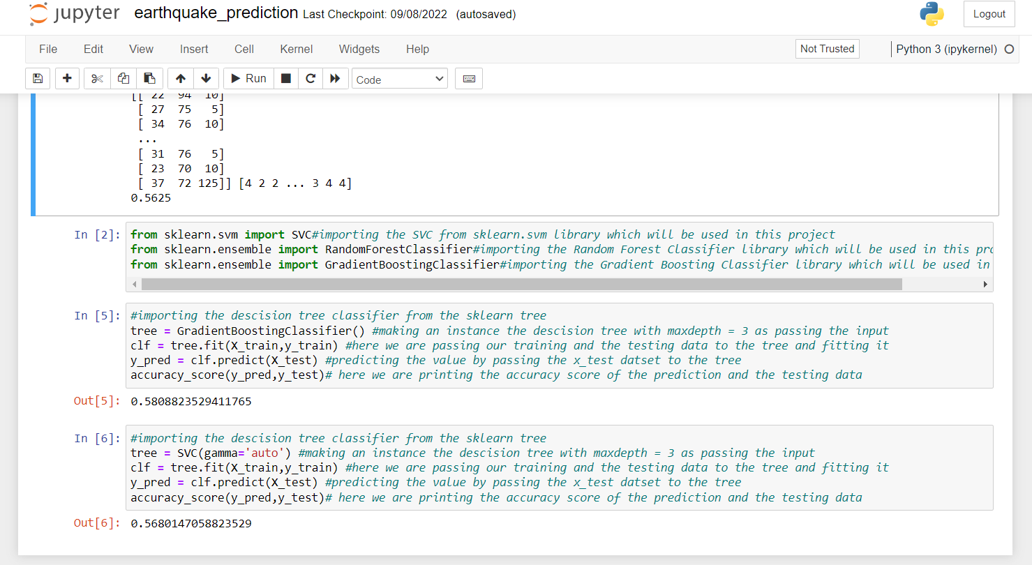
5. In this piece of code, we are creating our instance for Gradient Boosting Classifier. The maximum Depth of this Gradient Boosting algorithm is 3. After creating the instance, we pass our training data to the classifier to fit our training data into the algorithm. This is a part of training.

Once we are done with training, we pass the testing data, and we make our predictions on testing data and store it in another variable. After training and testing, it’s time to print the score. For this, we are using the accuracy score function, and we are passing the predicted values and the original values to the function, and it is printing the accuracy.

#importing the descision tree classifier from the sklearn tree 
tree = GradientBoostingClassifier() #making an instance the descision tree with maxdepth = 3 as passing the input
clf = tree.fit(X_train,y_train) #here we are passing our training and the testing data to the tree and fitting it

y_pred = clf.predict(X_test) #predicting the value by passing the x_test datset to the tree 
accuracy_score(y_pred,y_test)# here we are printing the accuracy score of the prediction and the testing data

6. Here, we are doing the same thing as above. The only difference is that this time, we are using Support Vector Classifier. So, we are creating an instance of Support Vector Classifier and setting the gamma function to “auto”. After that, we pass the training data to the classifier.

After training the model, we pass the testing data to our model and predict the accuracy score using the accuracy score function.

#importing the descision tree classifier from the sklearn tree 
tree = SVC(gamma='auto') #making an instance the support vector tree
clf = tree.fit(X_train,y_train) #here we are passing our training and the testing data to the tree and fitting it

y_pred = clf.predict(X_test) #predicting the value by passing the x_test datset to the tree 
accuracy_score(y_pred,y_test)# here we are printing the accuracy score of the prediction and the testing data

Summary

In this Machine Learning project, we built an earthquake prediction system. In this project, we used Random Forest Classifier, SVC, and Gradient Boosting algorithm in this project. We hope you have learned something new from this project.