VLOOKUP in Excel with Examples

Vlookup is a built-in function in MS-Excel. Vlookup stands for vertical lookup. In this vlookup function, it fetches the value from the column you specify.

In simple terms, we could say that vlookup helps to find the value you are searching for.

Vlookup parameters

Let’s know what are all included in the VLOOKUP function:

=vlookup(lookup value, table array, column index number, range lookup)

Let’s have a clear understanding about the parameters:

1. Lookup value

In this, you will enter something relevant to the value you’re searching for.

2. Table array

In this, you will enter the table value from where the search key should start its search.

3. Column index number

In this, you will enter the number of the column from which the lookup value should match and bring that particular column value.

4. Range lookup

In this, you will enter whether the search value should retrieve the approximate match or an exact match.

If you want an approximate match, then enter the value as 1, which represents true there.

If you want an exact match, then enter the value as 0, which represents false there.

Note: If you don’t enter the range lookup, then the parameter defaults it to 1, making an approximate match from the table.

Let’s look at the difference between an approximate and an exact match with a sample.

Approximate Match in Vlookup

As mentioned above, the approximate match works in an ascending order table. So, if you are going to make an approximate match, make sure your table is in ascending order.

Let’s look at a sample:

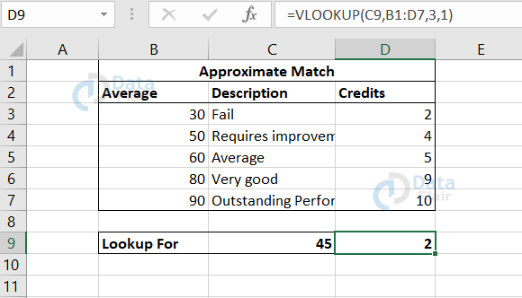
In the above sample, we can see that the table is already arranged in ascending order.

Now, we are going to fetch the approximate value for a student who scored 45%. This approximate match could be very useful because not every student could get 30, 50, 60, 80, or 90 percent marks. There can be fluctuations in it.

So, in order to decide on those fluctuated percentages, we can use vlookup with an approximate match.

This approximate match works even when the lookup value doesn’t match the table lookup value. If the lookup value is the mid of some two values, then it fetches the value with the smallest range among it.

The approximate match is also known as the closest match as they fetch the closest value for the lookup value.

In the above sample, we have looked up for the value of 45% and since 45 is not exactly available in the table, then the lookup value sees where this value lies.

As 45 lies between 30 and 50, the credit corresponding to 30 will be updated in the vlookup value cell. This is how the approximate match works.

If there is no provision of range lookup, then the parameter itself considers it to be as 1.

Let’s see a sample where we don’t give the range lookup parameter in the function:

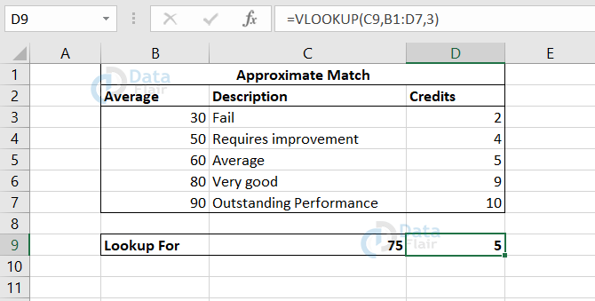
In the above sample, look at the function in the formula bar.

In the function, there are only 3 parameters that are being mentioned and the last parameter is not given.

But still, the vlookup function performs the action without throwing an error. This is because the default value of range lookup is 1 and if we don’t mention it in the parameter, then the function considers it to be as 1 and starts performing an approximate match.

For the above sample, we have looked up for the 75 percentage, and though we haven’t entered the range lookup, it went on with the approximate match and fetched the value as 5 in the D9 cell.

Exact match in Vlookup

In the exact match, the lookup value we have entered is being searched in the table and it returns the value only when there is an exact match.

Let’s look at a sample:

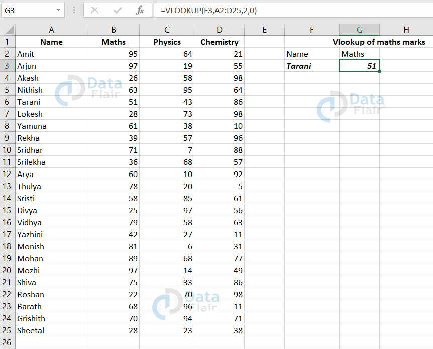
In the above sample, we have entered the range lookup value as 0 which represents to lookup for the exact value match.
Here, the lookup value is Tarani.

The table range is from A2:D25 and the column index provided is 2 which means we are looking for maths marks.
Then, the 0 represents the exact match from the table.
As we have provided the parameters, the maths mark is being fetched from the table that appears in the G3 cell.

How to use Vlookup in Excel?

Let’s see how to implement vlookup in MS-Excel:

Method 1

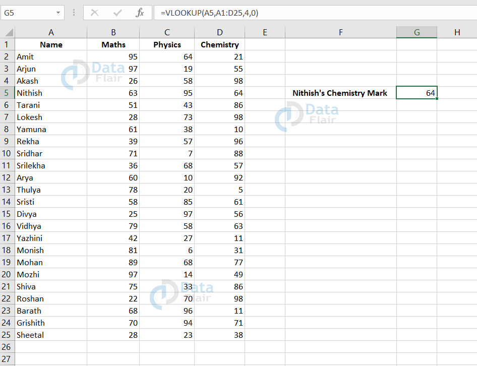
In the above sample, we have a list of students with their maths, physics, chemistry marks. Now, in order to search each and every value, we can just use the vlookup function to lookup a mark. This is what is being performed in the G5 cell.

Using vlookup function, we have fetched the Nithish’s chemistry mark in it. In the function, we have specified the name cell value as the lookup value.

A1:D25 denotes the table array.
4 represents the column number from where the value should be fetched.
0 represents the exact match.

After writing the function completely, Nitish’s chemistry mark is being taken from the table and it is shown in the G5 cell.

Method 2

There is also another way to make use of this function. You can either directly write the formula or if you are not sure about the formula, then follow the steps:

1: Click on the Formulas tab.

2: Choose the insert function.

3: A box appears with the list of functions. Hence, you can search for the vlookup in it.

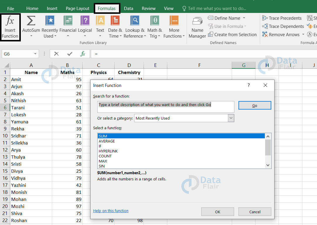
4: Select the vlookup from the list.

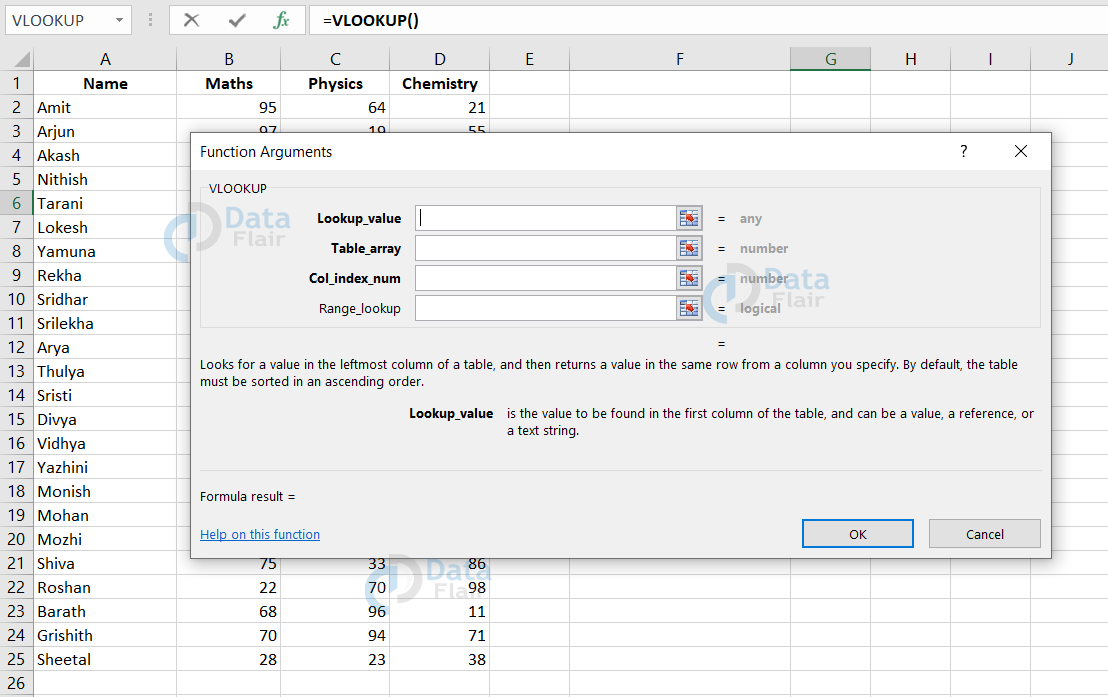
Now, when we clicked on the vlookup function, a box with its function arguments popped up.

5: Fill the details as per you are looking for.

6: Press ok.

Let’s look at a sample.

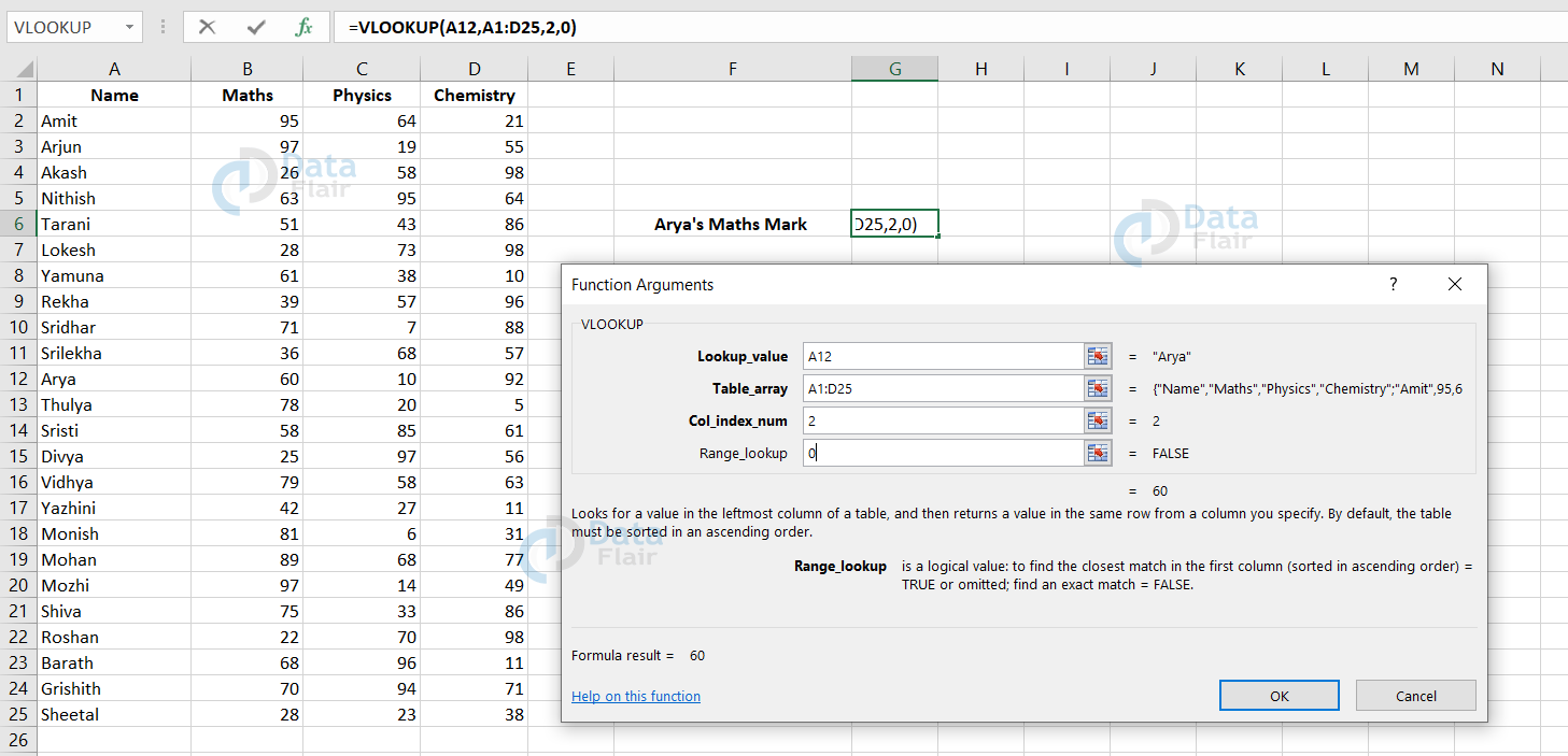
In this sample, we are trying to fetch the math’s marks of Arya from the table. To do so, we have filled the function arguments in the box. In the lookup value we have entered it as A12 as arya name appears there.

Here in the table array, we have filled it with the table range i.e., from A1:D25. In the col_index_num, enter the maths column number i.e., 2 in this table. In the range_lookup, fill it as 0 as we are looking out for an exact match.

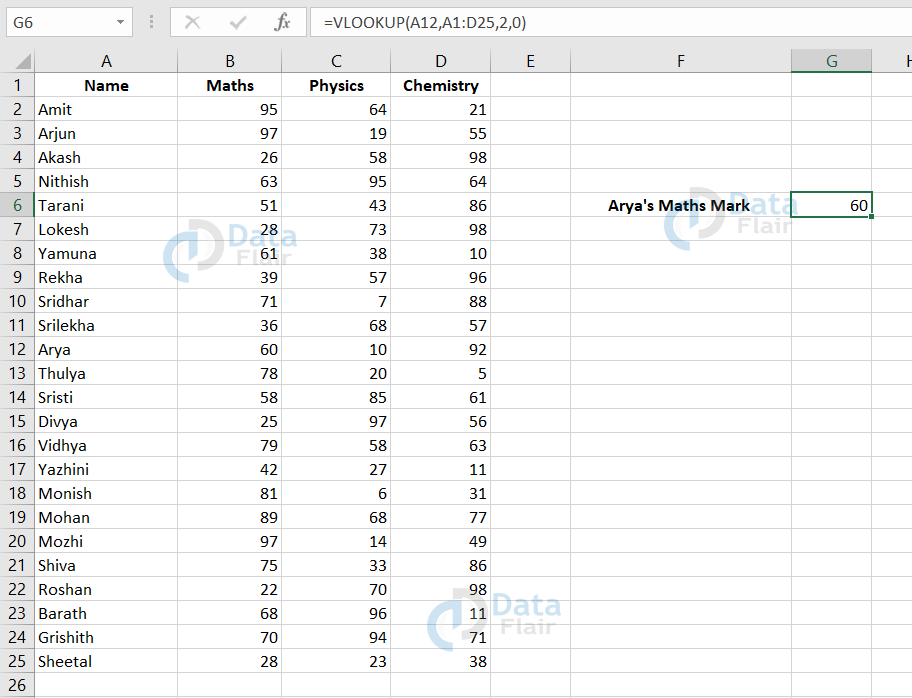
Now, after entering the values and once we press the ok button, the value is being fetched from the table and shown in the G6 cell.

Vlookup function with Data validation

Let’s see how data validation can help us in vlookup function. From the data validation, we are going to use the list option from it.

To utilize the data validation list option

• Click on the data tab.
• Choose the data validation and click on the list in the box.

Enter the source as which should appear as the list from the table. Now, apply the vlookup formula.

We use this data validation list option because it helps in saving our time by not typing the lookup value. Just a click on the list would fetch the required value from the table using vlookup function.

Let’s look at a sample.

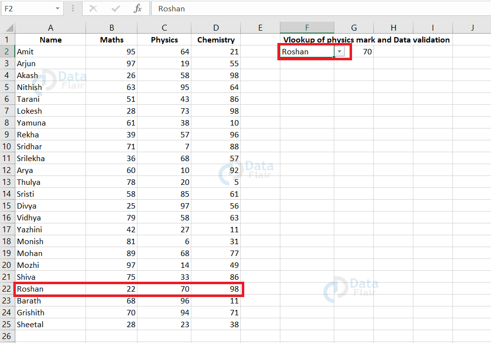
So, here we have made the list as names using data validation and we have used the vlookup function to lookup for the marks.

Now using the same list we will know whether the marks change if we change the name chosen in the list.

For that, let’s look into a sample where we have chosen the different name now:

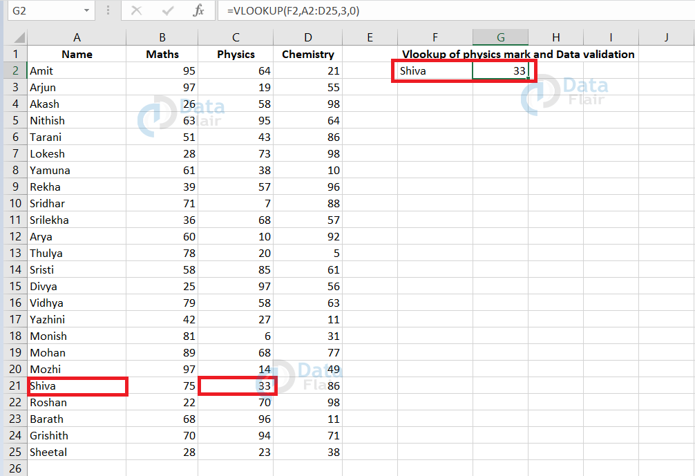
From the above sample, we can see that the vlookup value is being changed as the name changes.

Now you may wonder how this is possible. To understand it, have a keen look at the formula in the formula bar. We have written the formula as ‘=VLOOKUP(F2,A2:D25,3,0)’.

Here, we have mentioned the lookup value as the options we choose and that’s why it changes the marks accordingly.

Vlookup with formula

Let’s look at how vlookup function works with formula. It automatically updates with the value when the vlookup value changes.

For clear understanding, let’s look at a sample:

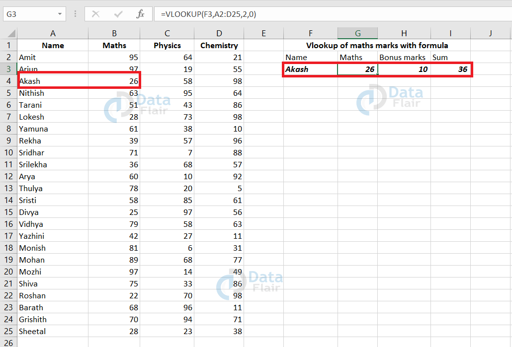
In the above sample, we are adding 10 marks extra to the maths marks we look up for.

Now, we have looked up Akash Maths marks in G3 cell and we have added 10 marks with it. The result of the sum value is in the I3 cell.

Now, even when we change the name in the lookup value, then for that lookup value also, 10 marks will be added on in the I3 cell.

Let’s have a look at it also.

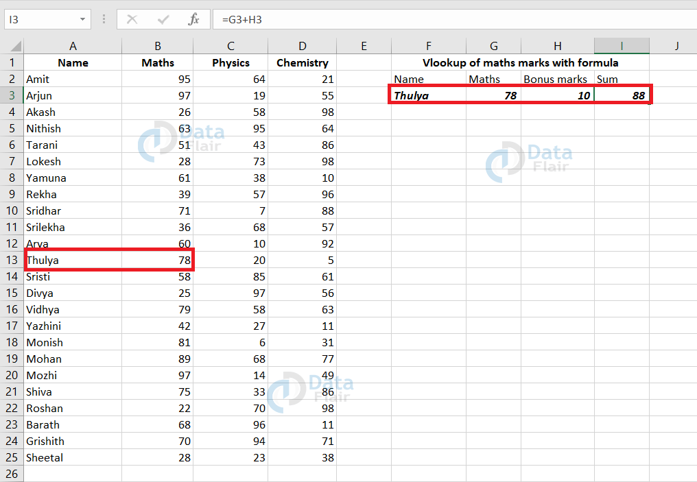
When we changed the lookup value as Thulya, then the maths marks of thulya is being fetched and bonus marks of 10 is added. This is being displayed in the I3 cell. The value automatically gets updated because it does not depend on the values. It depends on the cell number we have entered to calculate in it.

First Match in Excel

This is one type of vlookup. In the first match of vlookup, it matches with the first value it sees with the exact match. This applies when we have duplicate data in the table range.

Let’s look at a sample:

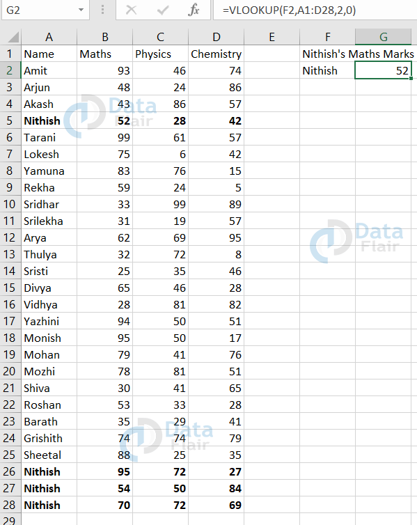
From the above sample, we could see 4 data rows in the spreadsheet with the name ‘Nithish’.
Now, when we look up the Nithish’s Maths marks then it fetches the data from the cell B5 since its first while searching.

Wildcard Match in Excel

Wildcard match is a match that works with a partial match in the search on a lookup value. But in order to do partial matching, you have to enter the range lookup as 0 to do an exact match.

Let’s look at a sample for clear understanding:

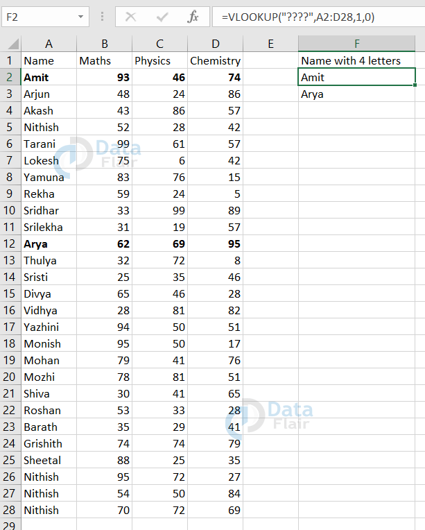
In the above sample, we have entered the formula as =VLOOKUP(“????”,A2:D28,1,0). This “????” represents that the value we are looking up is the 4 letters name of student.

Two-way VLookup in Excel

Until now, we have seen how a vlookup works when the column index is being provided. But now, let’s have a look at the sample where the column index is replaced by the match parameter.

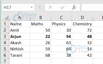
In this sample, we are going to look for the student whose name is Arjun and whose maths marks is 22.

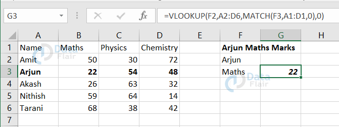
Look at the formula applied in the cell G3 in the formula bar. Here, we haven’t mentioned the column index. Instead, we will use a match function.

Here, we have written the formula as =VLOOKUP(F2,A2:D6,MATCH(F3,A1:D1,0),0)

F2 denotes which value we are looking for i.e., Arjun here.

A2:D6 denotes the table range.

MATCH(F3,A1:D1,0) – This denotes that the column index name is Maths which we are looking for in the F3 cell.

A1:D1 – denotes that these are column index headers.

0 here represents to make an exact match in the column header.

The 0 after the match function also denotes to make an exact match for the whole vlookup function.

VLOOKUP providing multiple criteria

In this function, there is no constraint that we have to provide only one lookup value. Instead, we could add multiple criteria using the “&” symbol in between. Now, let’s have a look at a sample:

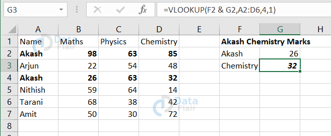
In this sample, we are fetching Akash’s chemistry marks providing his name and math marks as the lookup value. In this dataset, we have two students with the name Akash. So, we are providing the maths marks also to fetch the exact student we are looking for.

IF VLOOKUP in Excel

“If vlookup” function helps in calculating and comparing the values that we get by the vlookup. Let’s now look at a sample of how the if function works along with vlookup function.

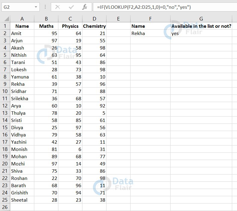
In the above sample, we are going to check whether the student name in the F2 cell is available in the list or not. In order to check this, we are going to use the if vlookup function.

Observe the formula in the formula bar. In that function, we have given all the input parameters for vlookup and yes or no is the value that results once we press enter.

As the student named rekha is available in the A9 cell in the list. Hence, the final result obtained is yes in the G2 cell.

Comparing Two lists using vlookup in Excel

Now, we are going to look at how vlookup function could help in comparing two lists.

Let’s analyze this with a sample:

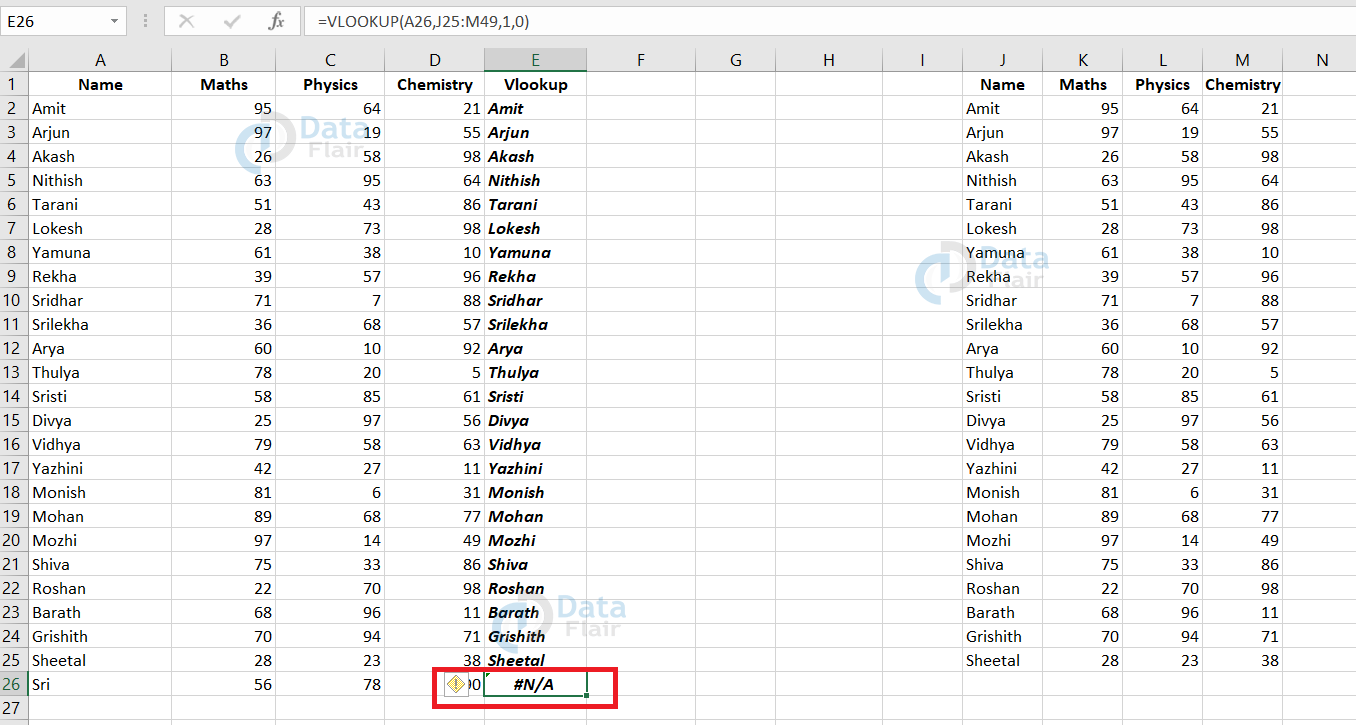
In this sample, we have two tables. One table is of the range A1: D26 and the other table is from J1: M25. Now, we are going to compare whether all the names of the students are available in both the lists or not.

To do so, we can use vlookup function to compare the lists. Here, the vlookup value gives back the name of the student itself if they are present in both the lists.

There is an error in the E26 cell and it’s because the marks of the student Sri is not available in the second table. That’s why there is an error as “#N/A” corresponding to the name Sri.

N/A errors:
Reasons Behind errors in Vlookup in Excel

• N/A errors appear when the lookup value couldn’t find the data in the table range.
• If the lookup value is misspelled or table range is not mentioned properly, There are high chances of error to occur.
• Even the range lookup value plays a vital role. The match value should be entered as per the requirement in the lookup.
• The error can be solved in the vlookup using IFNA function. This IFNA function helps in knowing from where the mistake is. IFNA function is being used to return a custom message if the cell is about to throw an error. 

How can we overcome the Vlookup error

• Make sure you don’t make a spelling mistake or a typo while typing the lookup value.
• Avoid using approximate matches when the data are not in ascending order.
• Make sure the lookup value is not smaller than the smallest value in the lookup array.
• If you are working on exact matches, then make sure that value is surely available in the dataset.
• Make sure the lookup value is not the leftmost column of the table array.

Summary

From this tutorial, we have understood what vlookup in excel is and where all it can be used. Vlookup function is a builtin function in MS-Excel. It widely helps for the references and it fetches the value from a particular range in no time. It also helps in comparing the lists and it works along with data validation and other formulas also.