SUMIF Function in Excel

First of all, let’s understand what sumif means. The sumif is a function that sums the following cells if it matches the criteria. Sumif is one of the impressive functions in MS-Excel.

Things to know before working with SUMIF:

1. SUMIF function supports only one condition whereas SUMIFS function supports the multiple criteria.

2. When you use text as a condition, then enclose it with double quotes (“”).

3. Wildcard characters can also be a part of the sumif function. Some of the wildcard characters are ?,*

Let’s now look where and how the sumif function works in a spreadsheet.

SUMIF function in Excel

Syntax:

=sumif(range,criteria,sum_range)

The parameters in the sumif function are:

1. Range

2. Criteria

3. Sum_range

1. Range

This parameter holds the range of the cell numbers. This denotes from where to where the cells can apply this function. It is a required parameter.

2. Criteria

This parameter says which criteria should be added together. This is also a required parameter and this parameter can be of any type like number, text, logical operators and so on.\

3. Sum_range

It is an optional parameter. This parameter should be of the same size as range and this helps in adding the other cells which are not specified in the range.

Let’s look at an example of with and without sum_range:

With sum_range:

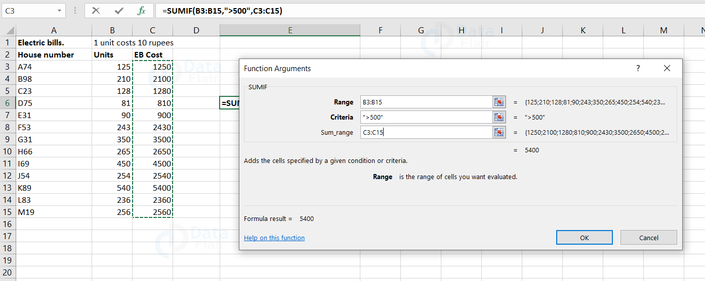
When we have sum_range in the function, then the function sums up the value from the cells we give in a sum_range. Let’s look at a sample:

In this sample, we have the dataset of house number, units and EB cost. Now, let’s calculate the EB cost of the houses which crossed the units consumption more than 500 i.e., >500

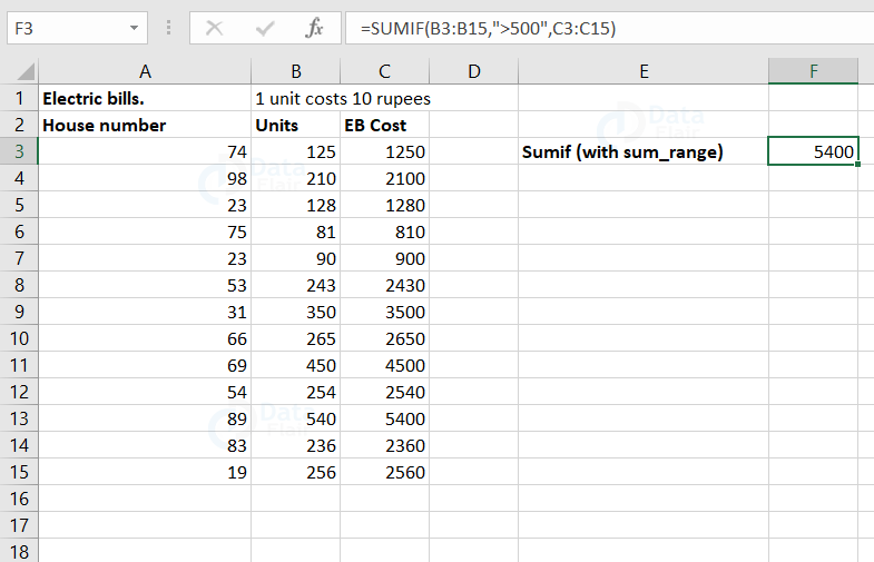
Here, we have given the cells from c3 to c15 as the sum_range.

Observe the formula of the cell F3 in the formula bar. The condition here says that the units above 500 in each house will sum up.

Since, we have only one house above 500 units then, that particular house EB Cost alone is being shown in the F3 cell.

Let’s look at another example.

Here, we will calculate the EB cost of the houses providing the criteria as the house number.

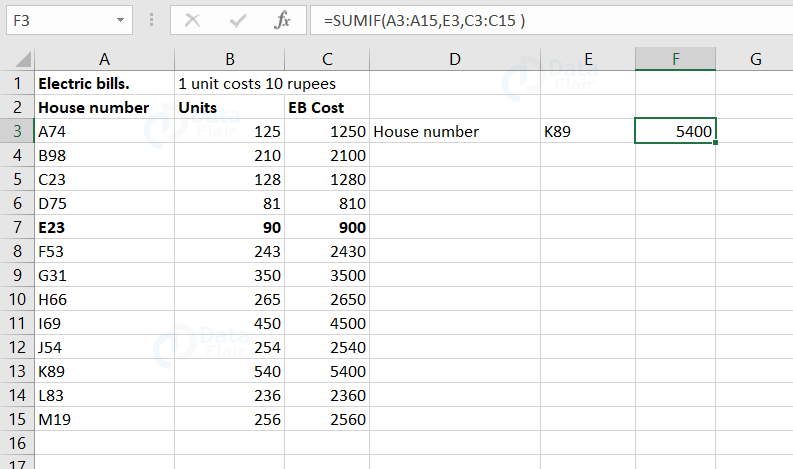
In this sample, we are calculating the EB cost of house number K89 and as there is only one house with that reference in the dataset, the function fetches that particular value alone.

Without sum_range:

When the user does not provide a sum_range parameter, then the calculation takes part for the range parameter itself. Now let’s look at a sample where we don’t provide the sum_range.

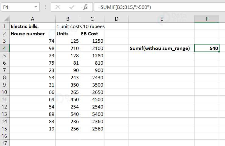
From the above sample, we can observe that the formula we have provided is : “sumif(B3:B15, “>500”) in the F4 cell. This function works in such a way that it sums up the value from B3: B15 if the units are above 500.

Hence, we have only one house more than 500, that particular house unit is alone shown in the F4 cell.

Methods of approaching the Excel Sumif Function

There are two ways to access the sumif function in a worksheet. One way is to directly write the function. The other way is to pick it from the formulas tab.

Follow the below steps to access sumif using the formulas tab.

1: Click on the formulas tab.

2: Click on the “Math & Trig”

3: Scroll down and choose the sumif function from it.

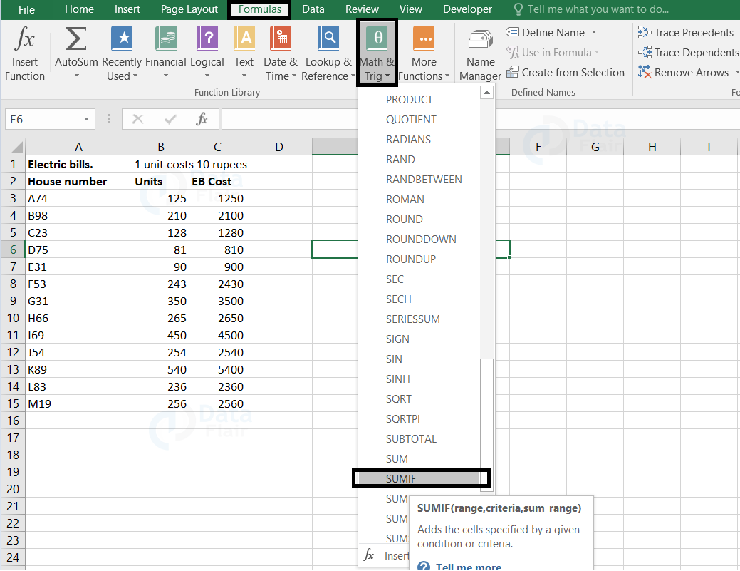
4: A box appears asking for the function parameters.

5: Fill the function parameters

6: Click on the OK button.

7: The answer will appear in the desired cell.

SUMIF Function Implementation

Now, let’s look at ways to implement Sumif Function:

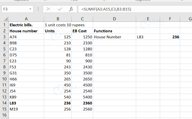
In this sample, we are trying to fetch the number of units consumed by the house number L83. In order to fetch it, we are entering the range as house numbers i.e., from A3 : A15 and the units column cells i.e., from B3: B15 as sum_range. The E3 in the formula bar represents which house we are looking at for.

Criteria in Another cell

Now, let’s look at the other sample where the criteria is mentioned in another cell.

In this example, sumif will return the sum of the units over the value in E3 cell.

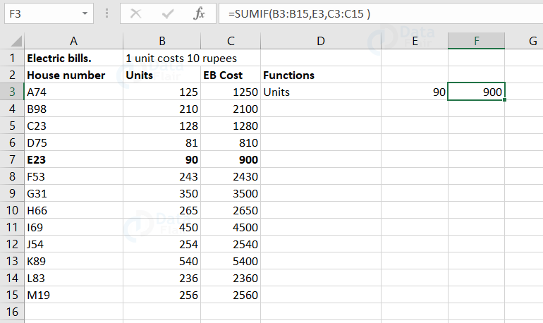
In this sample, we are fetching the EB Cost for the house which has consumed 90 units. Observe the formula of the F3 cell

in the formula bar. We have entered B3 to B15 as a range to look at and we are summing up the values from C3 to C15.

SUMIF with Comparison Operators

The advantageous part of sumif function is that it can perform calculations along with the comparison operators such as greater than or equal to, lesser than or equal to, great than, lesser than, equal to and not equal to.

Now, let’s see how logical operator performs in sumif:

1. Greater Than

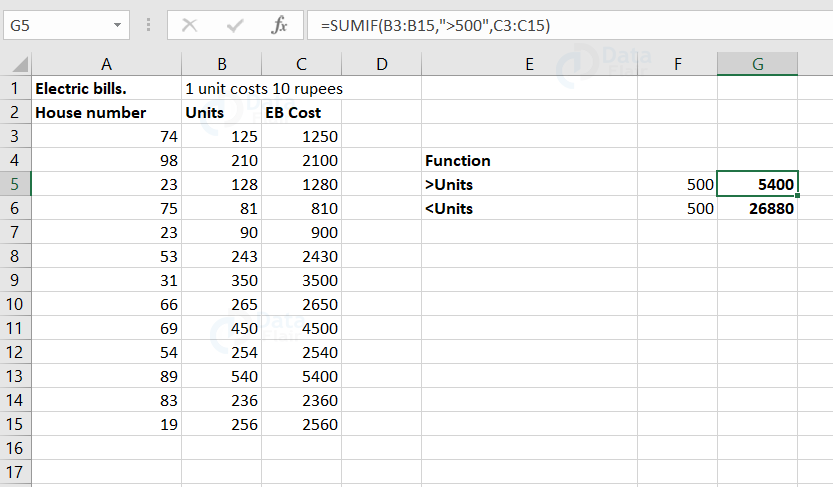
In this sample, at G5 cell, we are going to fetch the EB Cost of the house where greater than 500 units are being consumed.

Observe the formula of the G5 cell at the formula bar. We have provided the range as B3 to B15 cells, the condition in the quotation i.e., “>500” in this case. And we have provided the sum range as C3 to C15 here.

This means that the C column cells are being added if the B column cells meet the condition.

2. Less Than

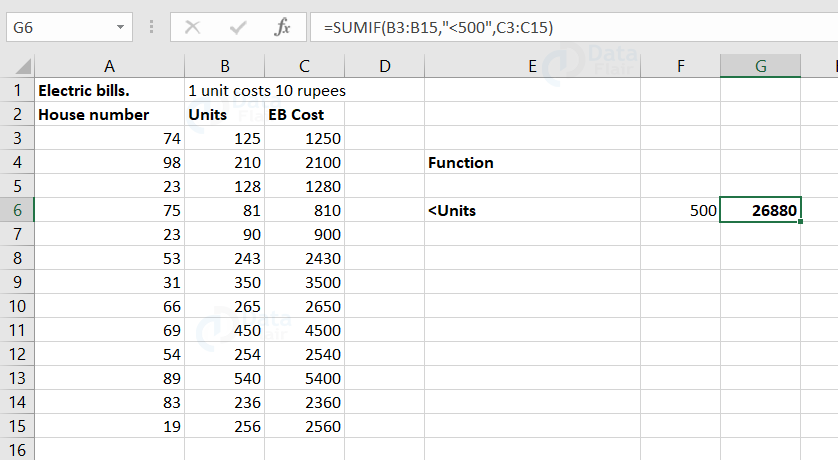
In this sample, at G6 cell, we are going to fetch the EB Cost of the house where less than 500 units are being consumed.

Observe the formula of the G6 cell at the formula bar. We have provided the range as B3 to B15 cells, the condition in the quotation i.e., “<500” in this case. And we have provided the sum range as C3 to C15 here.

3. Lesser Than Or Equal To

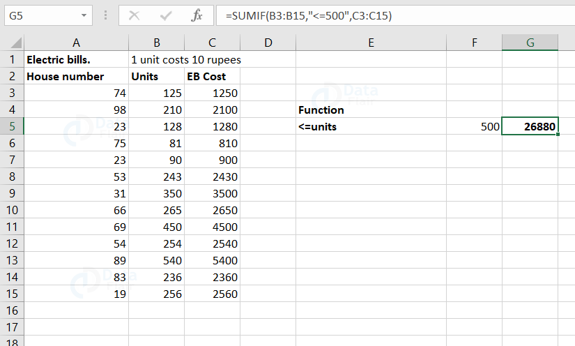
In this sample, at G5 cell, we are going to fetch the EB Cost of the house where the units are less than or equal to 500 units are being consumed. Observe the formula of the G5 cell at the formula bar. We have provided the range as B3 to B15 cells, the condition in the quotation i.e., “<=500” in this case. And we have provided the sum range as C3 to C15 here.

4. Greater Than Or Equal To

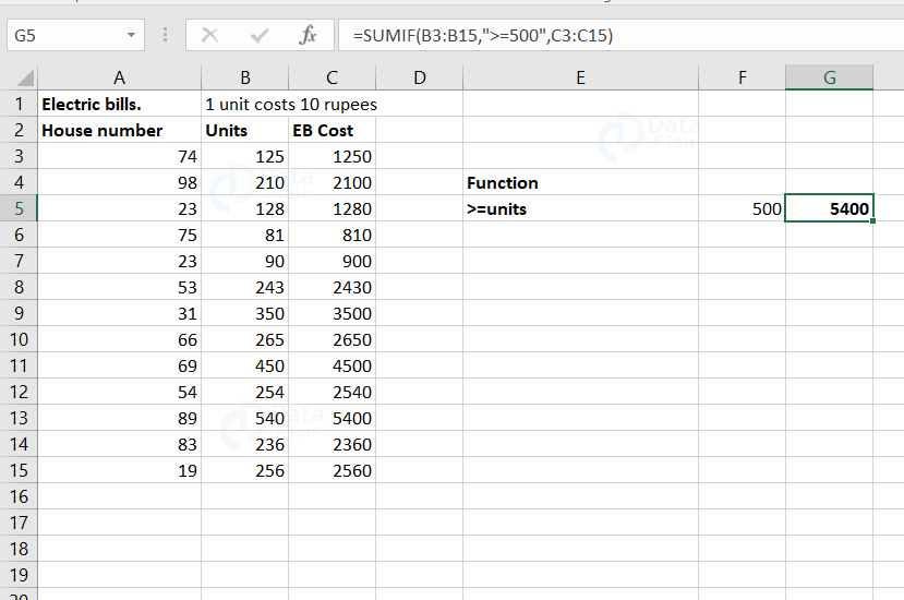
In this sample, at G5 cell, we are going to fetch the EB Cost of the house where the units are greater than or equal to 500 units are being consumed. Observe the formula of the G5 cell at the formula bar. We have provided the range as B3 to B15 cells, the condition in the quotation i.e., “>=500” in this case. And we have provided the sum range as C3 to C15 here.

5. Not Equal To

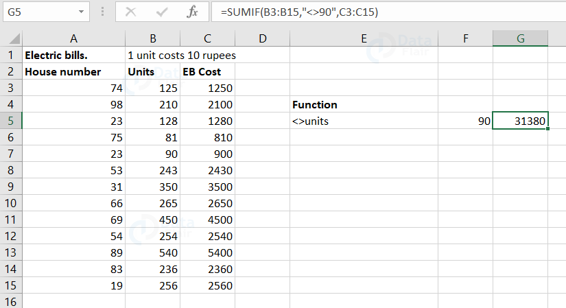
In this sample, at G5 cell, we are going to fetch the EB Cost of the house where the units are greater than and less than 90 units are being consumed.

Observe the formula of the G5 cell at the formula bar. We have provided the range as B3 to B15 cells, the condition in the quotation i.e., “<>90” in this case. And we have provided the sum range as C3 to C15 here.

Here, it means that all Eb costs of the houses are being added other than the 90 units consumed.

6. Blank Cells

The SUMIF function also performs its calculation based on the empty and non-empty cells. Let’s look at a sample.

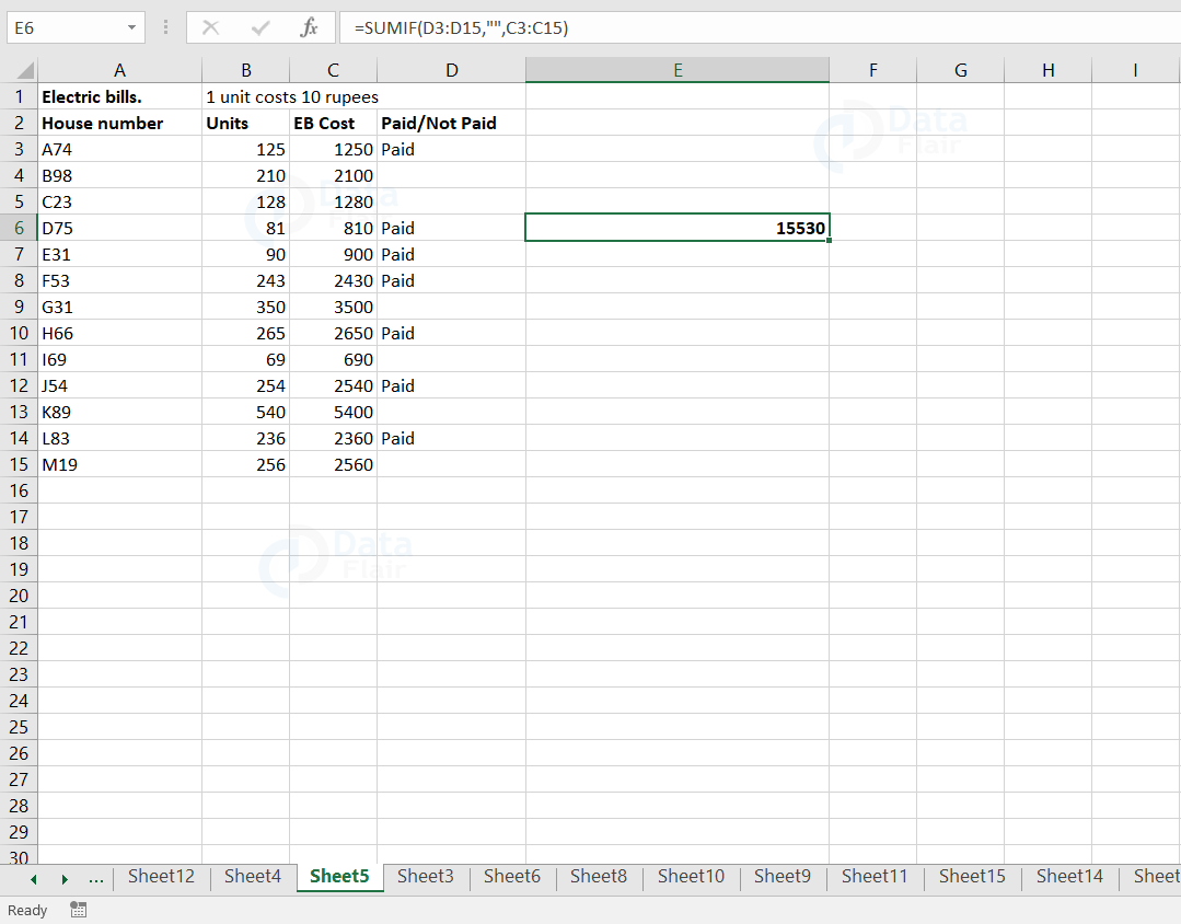
In this sample, at E6 cell, we are going to fetch the EB Cost of the house who has not paid the EB Cost yet. Observe the formula of the E6 cell at the formula bar. We have provided the range as D3 to D15 cells, the condition is a blank quotation i.e., “” in this case. And we have provided the sum range as C3 to C15 here. The blanks represent that those particular houses haven’t paid the EB bill.

Using Date as criteria

Date can also be a part of the sumif function. Now, let’s look at a sample of how the dates play a role as criteria in sumif.

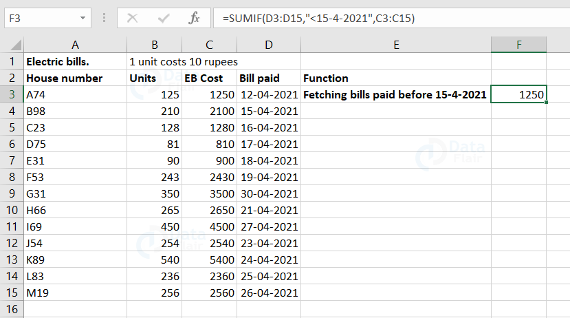
In the above sample, we are trying to use the dates as our criteria to check upon. In this, we are trying to sum up the bill if it is paid before 15th of april. Since, only one bill is paid before 15th of April, that bill amount is alone shown in the F3 cell.

Sumif between two dates

Using sumifs function, we can calculate the sum between two specific dates. It is a useful function to calculate the total of some specified range between any two dates. The main difference between sumif and sumifs function is that in sumifs function, you will have to add more than one criteria in a single function whereas sumif function accepts only one criteria in a function.

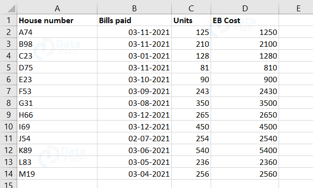
As we can see, the bills paid column has different dates. Now with the help of Sumifs, we need to calculate the sum of the EB Cost in between two dates.

For this, we need to select two dates between the dates mentioned in bills paid columns in separate cells. Before that, let’s understand the syntax of Sumifs function:

Syntax: SUMIFS(Sum_Range,Criteria_Range1, Criteria1…)

Sum_Range = Sum range or date which needs to be added.

Criteria_Range1 = This is the first criteria range for which we are going to get the sum. There can be one or more criteria.

Criteria1 = This is the first criteria under which basis we will calculate the sum output. There can be more than 1 criteria in this also.

Note: Ampersand (&) in criteria1 and criteria2, we use ampersand (&) for concatenating the dates with these “<=” , “>=” signs.

Now let’s apply Sumifs and calculate the sum between two dates.

Example-1:

Syntax:

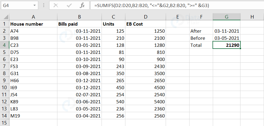
SUMIFS(D2:D14,B2:B14, “<=”&G3,B2:B14, “>=” &G2)

Observe the formula in the formula bar. Here, we have selected the Sum Range as D2 to D14, Criteria Range1 as B2 to B14. Now for criteria1 add “<=”&G3 (After Date 3-11-2021). In the next phase, select the criteria Range2 again as B2 to B14 and for criteria2 add “>=”&G2 (Before Date 03-05-2021). Hence, the total is calculated between those two dates.

Example-2:

Syntax:

SUMIFS(D2:D14,B2:B14, “<=03-11-2021”,B2:B14, “>=03-05-2021” )

Here, we are not using the ampersand and it’s because we are directly specifying the date in the formula rather than providing it with a cell reference.

Note: We use ampersand (&) only when we provide the dates as cell reference.

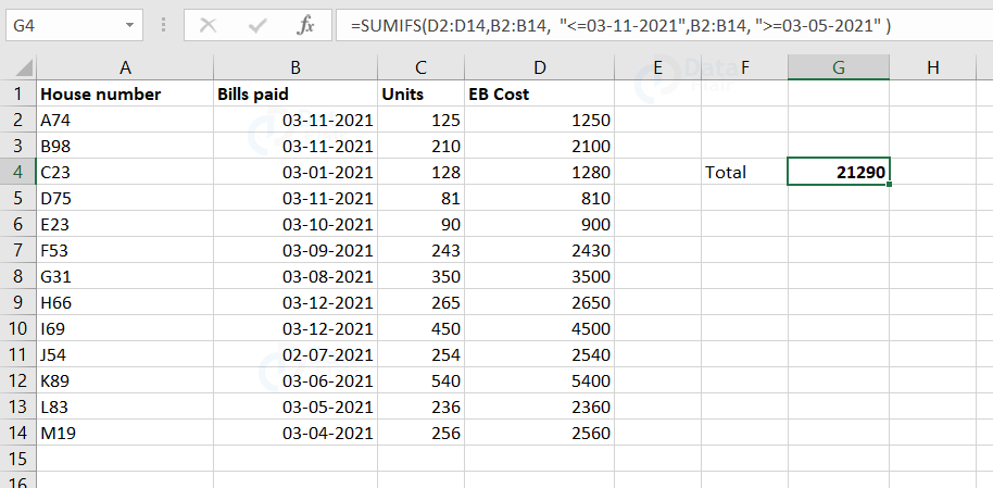
The formula calculates the EB Cost which is paid between the 03-05-2021 and 03-11-2021 in the G4 cell.

Pros of Sumif between two dates:

1. We can calculate the sum of a specific column between selected dates.

2. The syntax might look a bit difficult but the implementation is quite easy.

3. After and before dates can be changed as per the convenience.

Cons of sumif between two dates:

1. Sometimes, there are chances of obtaining the final result as 0 and this is mainly because the user may interchange the before and after dates.

2. Before executing the formula, make sure the date column is in the date format.

Things to Remember

1. Select the before and after date in sequence.

2. The first half syntax contains the after date and the other half syntax contains the before date.

3. Single date calculates the result specific to that date only.

4. Make use of Ampersand to concatenate the dates with criteria as dates are chosen by selecting specific cells.

Sumif with Text:

The sumif function can also perform the calculations by considering the condition as text. Let’s look at a sample to understand this concept.

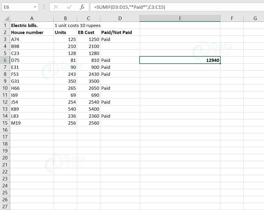
In this sample, at E6 cell, we are going to fetch the EB Cost of the house who have paid the EB Cost. Observe the formula of the E6 cell at the formula bar. We have provided the range as D3 to D15 cells, the condition in the quotation is “*Paid*” in this case. This means that we are trying to sum up the EB costs of the houses who have already paid. And we have provided the sum range as C3 to C15 here.

Wildcard in sumif function:

The sumif function can also perform calculation by making use of the wildcard characters such as *,? in the arguments. Let’s look at an example.

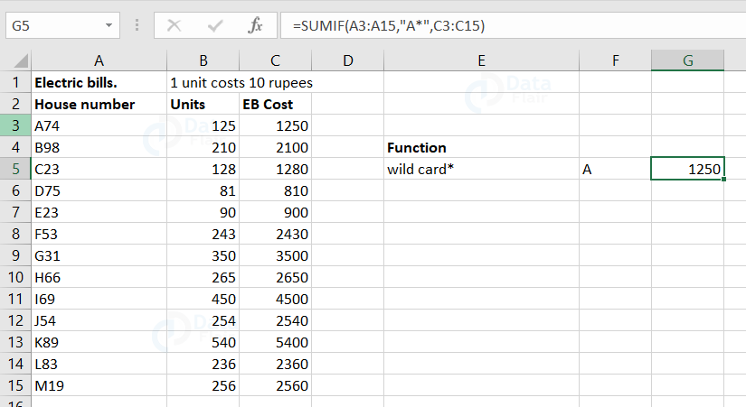
In this sample, at G5 cell, we are going to fetch the EB Cost of the A block house.

Observe the formula of the G5 cell at the formula bar. We have provided the range as A3 to A15 cells, the condition in the quotation is “A*” here in this case. This means that we are trying to sum up the EB costs of the houses starting with A. And we have provided the sum range as C3 to C15 here.

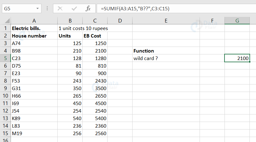
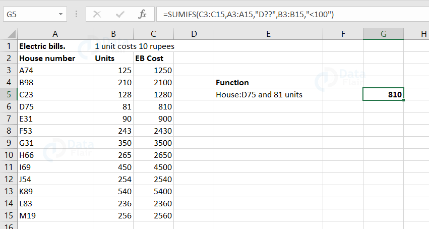
In this sample, at G5 cell, we are going to fetch the EB Cost of the B block house.

Observe the formula of the G5 cell at the formula bar. We have provided the range as A3 to A15 cells, the condition in the quotation is “B??” here in this case. This means that we are trying to sum up the EB costs of the houses starting with B and being followed by any values. And we have provided the sum range as C3 to C15 here.

Things to remember about sumif function with text:

1. The text must be enclosed in a double quotation(“ ”).

2. If the sum_range is not provided, then it computes the summation for the range cells.

3. The user can perform wildcard matches using a question mark(?) and an asterisk(*)

AND criteria in SUMIF Function

Let’s get into the concept of sumifs function . We use sumifs function when we have two or more conditions to meet its criteria. The sumifs function is applied with the AND logic to find if both the conditions satisfies.

Let’s look at a sample to understand this briefly:

In our sample, we are trying to add the EB costs of the house number starting with D?? and where the units are less than 100.

To write these conditions in a function, we use sumifs.

Observe the formula at the formula bar. Here, C3 to C15 cells denote the value which has to be summed up. The A3: A15 cells are given to check whether there are houses starting with D and also checking up on the units which are less than 100 in the B3 to B 15 cells.

OR criteria in SUMIF Function

The user can combine OR logic with sumif condition to sum the values using two or more different criterias at the same time.

Example- 1:

Let’s now look at a sample where we use one or more sumif in the same cell.

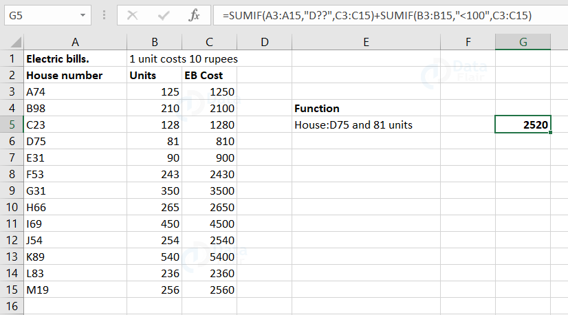
In our sample, we are trying to add the EB cost of the house number starting with D and where the units are less than 100.

To write these conditions in a function, we are going to use the sumif function twice.

Observe the formula at the formula bar. Here, C3 to C15 cells denote the value which has to be summed up. The A3: A15 cells are given to check whether there are houses starting with D and the cells B3 to B15 are given to check up on the units which are less than 100.

Example – 2:

Sumif with OR

In this sample, we are going to execute the calculation using sumifs function. Let’s look at the sample.

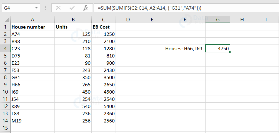
In this sample, we are calculating the EB Cost of the houses H66, I69 using sumifs function. Here, C2:C14 is the sum_range, A2:A14 is the criteria range and the values in the curly braces i.e., {“G31” , “A74” }are the criteria to satisfy.

Usually, the formula syntax is sum_range, criteria_range1, criteria1, criteria_range2, criteria2…

But here, we have made a lit bit of changes as the criteria range is the same for the defined criteria. We have used sum here in front of the sumifs to calculate the value for both criteria.

If we don’t use sum before the sumifs while entering the criteria as an array, then the result will be:

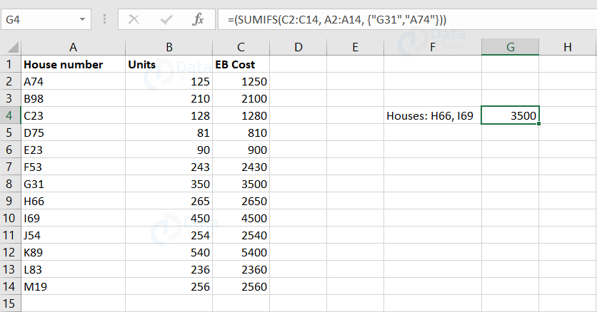
From this, we can understand that both the criterias are not met. When a criteria is met, the function stops performing and the rest criterias are left without any consideration. In order to overcome this issue, we use the sum function in front of the sumifs function.

Things to remember about sumif with or:

1. SUMIF follows the AND logic which means it performs summation if the criteria match.

2. SUMIFS will follow the OR and AND logic which means it can perform multiple criteria at a time.

Errors in sumif:

1. The value error throws up when the criteria range does not fall in the range of sumif function.

2. The name error is being shown when the order of the parameters is not followed.

Difference between the subtotal and sumif function:

Subtotal function applies on the filtered table data whereas sum if function executes on an ordinary excel spreadsheet. Both the functions are more or less the same, but the advantage of the sumif function is that it works on a normal spreadsheet satisfying the defined criteria. In simple terms, subtotal function computes the column data value when the filter is applied and sumif function computes the column data value even without the filter being applied in the spreadsheet.

Summary

Sumif sums as per the criteria provided. It works one column at a time. This function can work along with wildcard matches. It allows numeric and text data types.