PyTorch Linear Regression

Linear Regression is an ML algorithm that tries to find a linear relationship between the inputs and the outputs of the training set. Then, based on this learned information, it tries to predict the output of the test dataset. It is widely used in prediction models, such as housing prices prediction models, stock prices prediction models etc., when we have some knowledge about the past and the prediction we have to make is a real number.

What is Linear Regression?

In linear regression, our job is to fit the given data into a straight line. The equation of a line will be y=mx+c. Here, y is the dependent, and x is the independent variable of that data.

Our task is to find the parameters m and c. Once we have computed m and c, we can predict the output for any new input.

In machine learning, we replace the parameters c and m with Ө0 and Ө1. Now the equation becomes y=Ө0 + Ө1x. The advantage of this representation is that the parameters and the independent variable can be represented as vectors.

x=[1  x]^T                 Ө=[Ө₀   Ө₁]^T

And the equation of a line can be written as y=Ө.x.

If there are more than one independent variable, this representation can be extended.

x=[x₁  x₂  x₃  ………..  x_n]^T                         Ө=[Ө₁  Ө₂  Ө₃  …………….  Ө_n]^T ,here x₁=1

And the equation of the line remains the same.

                                              y=Ө  . x

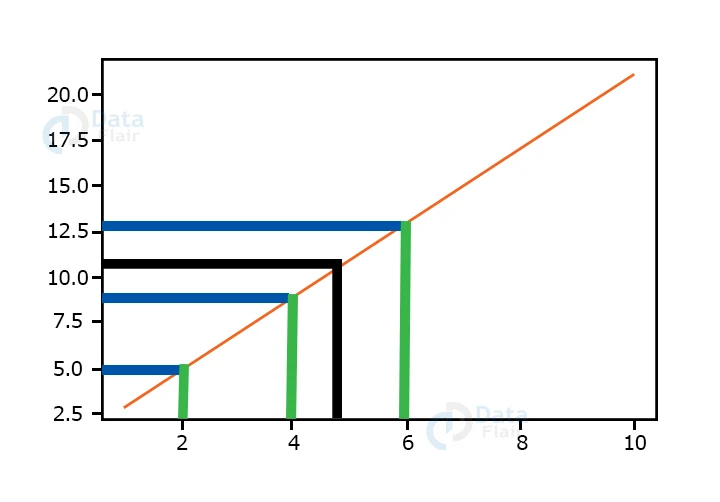
Suppose we have three (x,y) pairs. {(2,5), (4,9), (6,13)}. It is a simple example. To train our model, we need to find the vector Ө. Now, for any given x, we can easily compute the value of y. We plot the three training examples, which fall in a straight line in this case. If the given x is 5, we can find the y value using this plot.

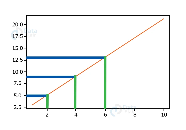
The parameters of this model can easily be calculated to be Ө₀=1 and Ө₁=2.
ஃ y=1 + 2x.

Using this learned information we can compute (predict) the output of any new input data.
For x=5, y=1+2*5=11.

This was a simple example, but actual tasks are not so easy. The training examples may be scattered yet they appear linear, and we will have to find the best fit.

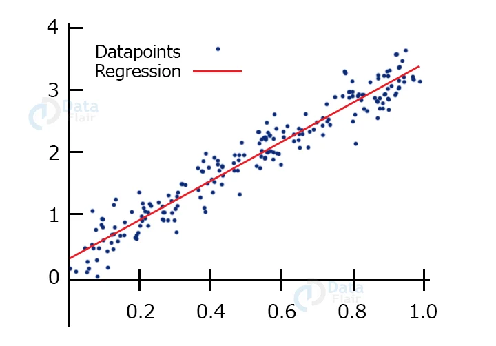
In this picture, the examples do not lie in a straight line. However, they seem to follow a line closely. This line can be the one that can fit the dataset with the least loss and hence be the required model.

Methods of finding the parameters of a model in Linear Regression:

1. Gradient Descent Method:

The parameter vector θ can be computed by plotting a loss curve, which will always be a parabola with its opening in the upward direction, then picking a point on the curve and moving towards the minimum of the curve to find the parameters’ optimal value.

We upgrade the value of the vector θ as follows.

θ _j:=θ _j-(α/m)*∑_i=1^m (h_θxⁱ–yⁱ)x_j

2. Normal Equation Method:

The normal equation method is a straightforward method of computing theta without requiring any loop and is, therefore, asymptotically faster.

Ө=(X^T*X)^-1.X^T*Y

Linear Regression using numpy:

We will try to build a linear regression model which uses the normal equation method to find the value of Ө.

a. Importing the required libraries

import numpy as np
import matplotlib.pyplot as plt
%matplotlib inline

b. Making dummy dataset

We will build our own dataset to train a regression model.

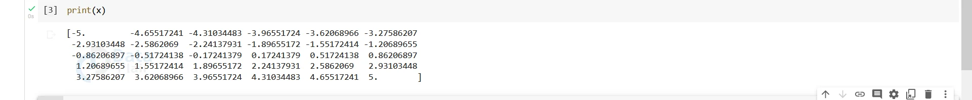
x=np.linspace(-5,5,30)
y=12*x

print(x)

Output-

print(y)

Output-

c. Adding noise to the output vector and reshaping the vectors

The dataset we have created is a straight line. To make it a bit more challenging, we will add some noise to it. The data thus created will resemble that in practical examples in terms of being scattered.

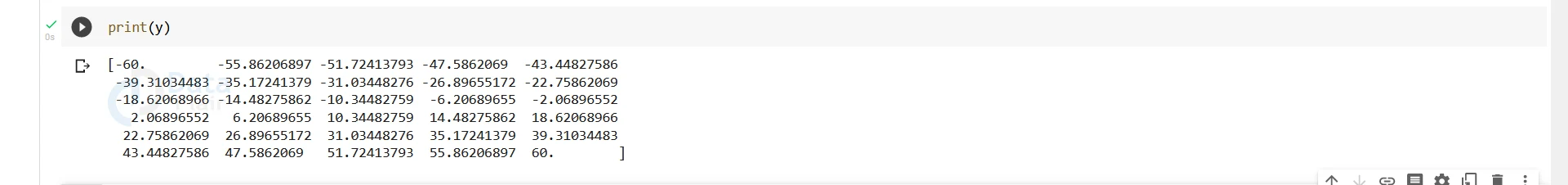
noise = np.random.normal(0, 5, y.shape)
y=y+noise

print(y)

Output-

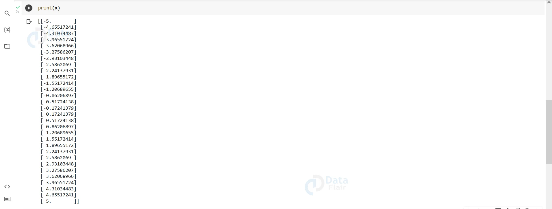
x=x.reshape(-1,1)
y=y.reshape(-1,1)
 
print(x)

Output-

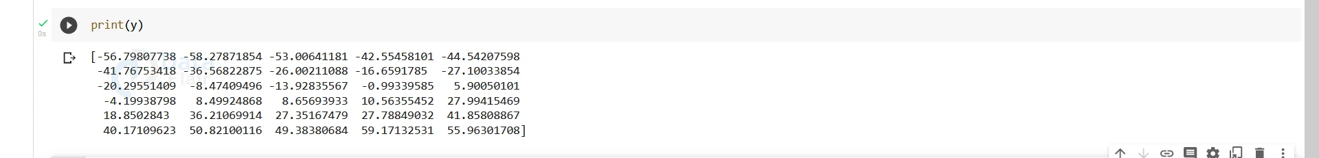
print(y)

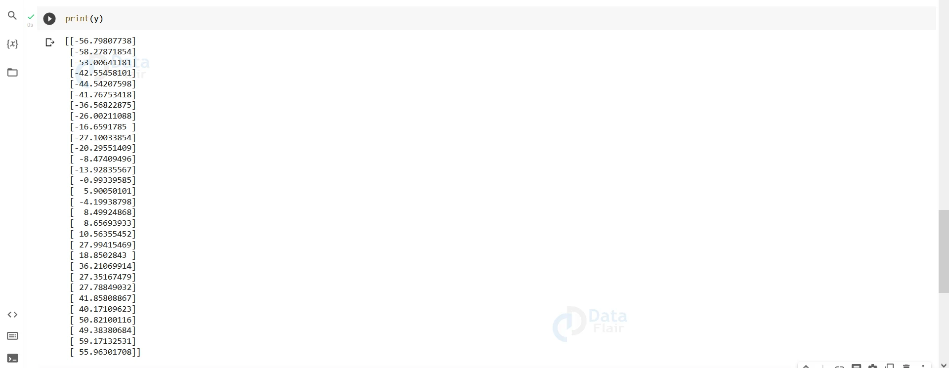
As we can see the vector y is no longer precisely linear to the input.

Every other pair of points has a different gradient and intercept. Our job is to find a line so that the distance betweeb these points from it is minimum.

d. Using the normal equation method to compute the parameters

For this example, we will use the normal equation to calculate theta.

theta=np.dot((np.linalg.inv(np.dot(x.T,x))),(np.dot(x.T,y)))

print(theta)

Output-

e. Visualising the prediction along with the input initial input and outputs

Firstly, we will plot the initial x and y. Then, plot the x and the y computed using the calculated theta (prediction). Finally, we will plot both of these graphs together to see if our prediction is good or not.

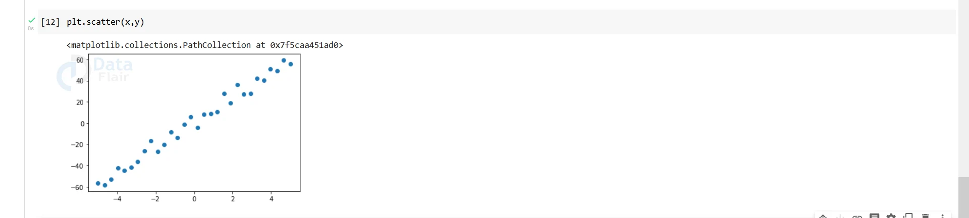
plt.scatter(x,y)

Output-

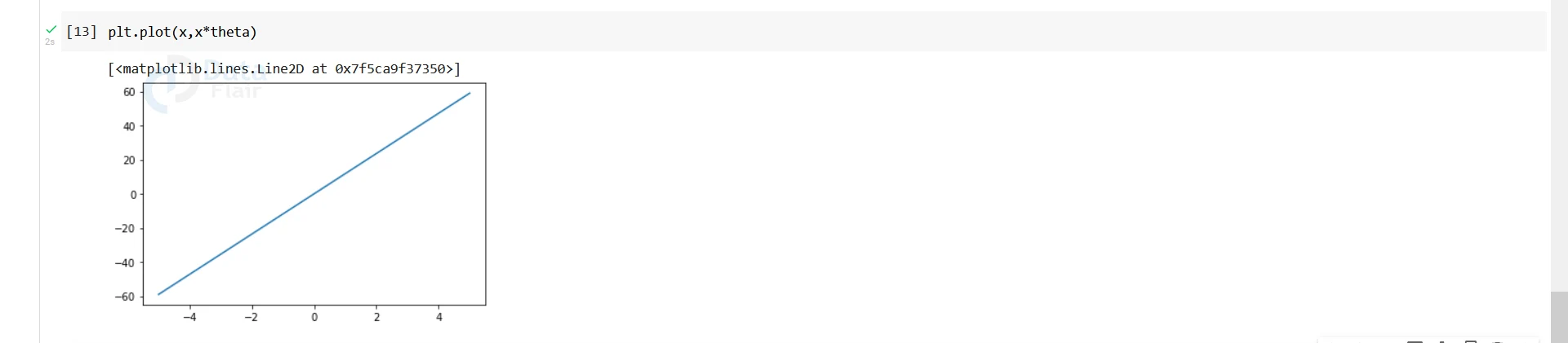
plt.plot(x,x*theta)

Output-

plt.scatter(x,y)
plt.plot(x,x*theta)

Output-

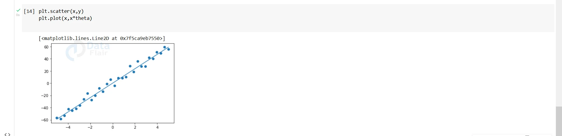
As we can see that the prediction curve follows the initial data points very closely, we can rest assured that our model is working properly.

Building Linear Regression Model Using PyTorch:

Now that we have built a model using numpy, we will try to build one using PyTorch. This time we will use Gradient Descent as the optimisation algorithm.

a. Importing the required modules

Before doing anything, we have to import torch and other required libraries.

import torch
from torch.utils.data import TensorDataset,DataLoader
import torch.nn as nn
import numpy
import matplotlib.pyplot as plt

b. Building the model

class Model(torch.nn.Module):
    def __init__(self):
    	super(Model, self).__init__()
    	self.linear = torch.nn.Linear(1, 1)

    def forward(self, x):
    	y_pred = self.linear(x)
    	return y_pred

lreg=Model()
#Creating an instance of the model we have created above

criterion = torch.nn.MSELoss()
#specifying the loss function. Here we have used Mean Squared Error Loss

optimizer = torch.optim.SGD(lreg.parameters(), lr = 0.01)
#Optimising the model using Stochastic gradient descent.

c. Preparing data

#Now we will create random data to train our model

x = torch.tensor(range(-5,5)).float()
y = 12*x

x_train = x[:,None]
y_train = y[:,None]

#We have taken the transpose of the input and output tensors to transform its shape from 1 x 10 to 10 x 1.

d. Training the model

for i in range(500):
   	 
    	optimizer.zero_grad()
    	#If we do not set grad to zero then the old gradients will add up in the current gradients making our model incorrect.
   	 
    	y_pred = lreg(x_train)

   	 
    	loss = criterion(y_pred, y_train)
   	 
    	loss.backward()

#Back propagating the neural network to find the gradient of the output with respect to the given parameters.

   	 
	optimizer.step()
	#Optimising the weights of the neurons depending on the gradient calculated during backpropagation.

	print(i,loss)

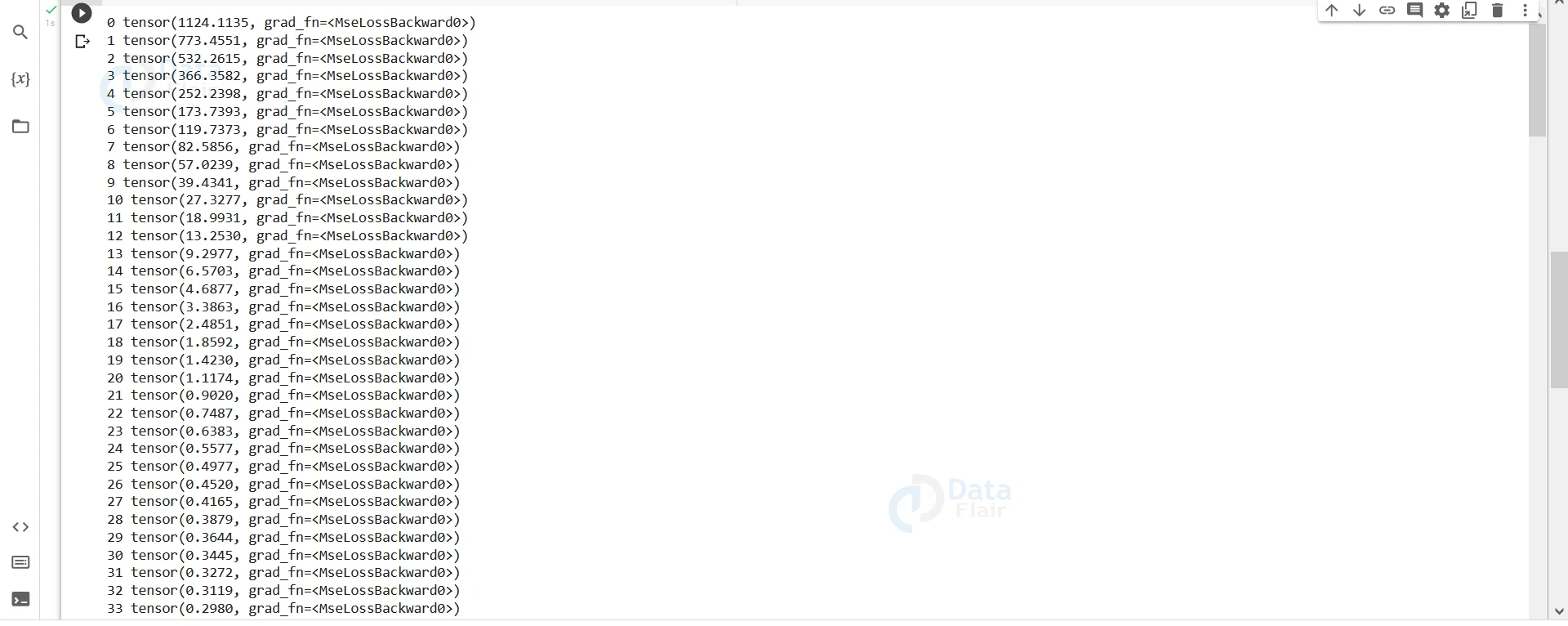
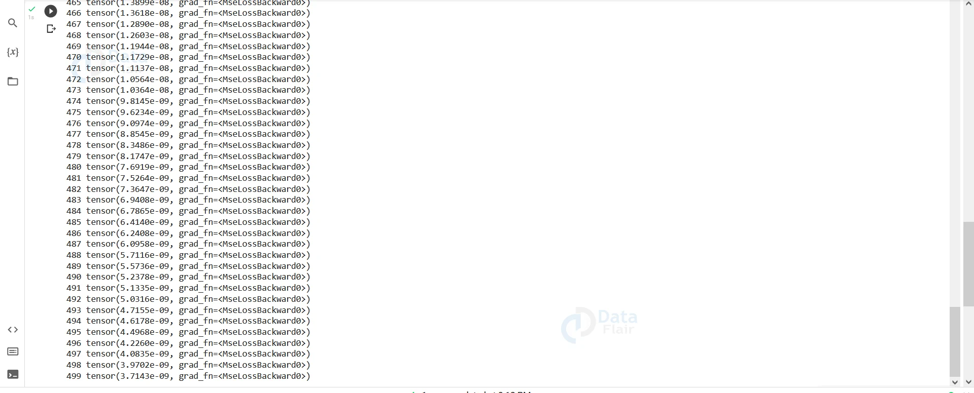
On running this part, we will see that the loss slowly decreases and comes closer to zero.

Summary

It is fascinating that we can use Neural Networks and PyTorch to build regression models because they were invented for classification problems. Models built this way often perform better than those built by other methods. To build a model using PyTorch, we have to import torch.nn, backpropagate and finally, optimise the network.