PyTorch CNN

CNN stands for Convolutional Neural Networks. Classification has been a popular application of Machine Learning. CNN models are good at detecting patterns and are therefore employed mostly for problems related to image classification/recognition, such as facial recognition of our smartphones. It detects patterns like edges, circles, bulges etc. and associates them to one of the outputs probabilistically, thereby learning different characteristics of different classes. In this tutorial, learn more about PyTorch CNN.

Why Convolution Neural Networks?

Convolution Neural Networks, as powerful as they are, are thought to have been inspired by the idea of mimicking the human brain. In fact, from a bird’s eye view, they perform functions similar to a human brain. Scientists in the 20th century proposed that our brain applies some filter to the image perceived by the eye to identify it. It is exactly how a convolution neural network works. However, the exact picture is somewhat different compared to an elementary level.

Another school of thought believes that it owes its popularity to its ability to identify patterns irrespective of the image’s scale or orientation. For example, suppose we train a model to identify a nose. Now, if we give an image of an entire face to our trained model, it will correctly identify the nose as it takes into account all the smaller fragments of the input independent of the remaining parts of the image. This property is also known as the regularisation mechanism of the convolutional neural network.

CNNs are also good at identifying images even when rotated or spatially altered. It is called the property of invariance.

Working of a convolution layer:

In a convolutional network, the hidden layers consist of multiple (not necessarily all) convolutional layers. These layers have some filters to extract information about patterns. It is done by convolving the filter matrix over the input matrix.

Suppose the input matrix is :

And the filter matrix is F:

The output of this layer will be an activation map obtained by convolving A with F. The convolution operation will be represented as A * F. Let’s try to understand this operation by applying it to the above matrices.

The number of columns of the activation matrix will be the number of submatrices of matrix A that can be overlapped by the filter matrix F in the horizontal direction.
Here, it will be 4.

Similarly, the number of submatrices of matrix A can be overlapped by the filter matrix F in the vertical direction. In this example, it will also be 4.

So, our activation map/matrix will be a matrix of dimension 4 x 4.

Now we will start convolving from the upper left part of the matrix A.

The elements of the activation map can be found as follows.

a₁₁ = (1*1) + (2*2) + (6*3) + (7*4) = 1 + 4 + 18 + 28 = 51

a₁₂= 2*1 + 3*2 + 7*3 + 8*4 = 2+6+21+32 = 61

Similarly, we can calculate all the values.

Resultant matrix will be

The filter matrices are designed so that the activation matrices obtained can help the network to identify some patterns in the input image.

Implementing a Convolutional Neural Network using Pytorch:

The good thing about PyTorch is that we do not have to hardcode all the convolution layers, nor do we have to implement the activation functions ourselves. PyTorch has some libraries that can be used for these tasks, as seen in the code example below.

a. The MNIST Dataset:

The MNIST dataset contains images of handwritten numbers from 0 to 9, making a total of 10 categories. Furthermore, it consists of all possible ways a person can write these numbers. Therefore, we can train our model using the MNIST dataset to identify handwritten numbers.

b. Importing the required libraries:

Firstly, we will import all the libraries which we may need for our model.

import torch
import torchvision
import torch.nn as nn
import torch.optim as optim
from torchvision import transforms,datasets
import torch.nn.functional as F
import matplotlib
import matplotlib.pyplot as plt

c. Loading the data:

train=datasets.MNIST("", train=True,download=True,transform=transforms.Compose([transforms.ToTensor()]))
test=datasets.MNIST("", train=False,download=True,transform=transforms.Compose([transforms.ToTensor()]))

trainset=torch.utils.data.DataLoader(train,batch_size=64,shuffle=True)
testset=torch.utils.data.DataLoader(test,batch_size=64,shuffle=True)

d. Playing around with the loaded data:

for i in range(5):
    print(train[34+i][1])

Output

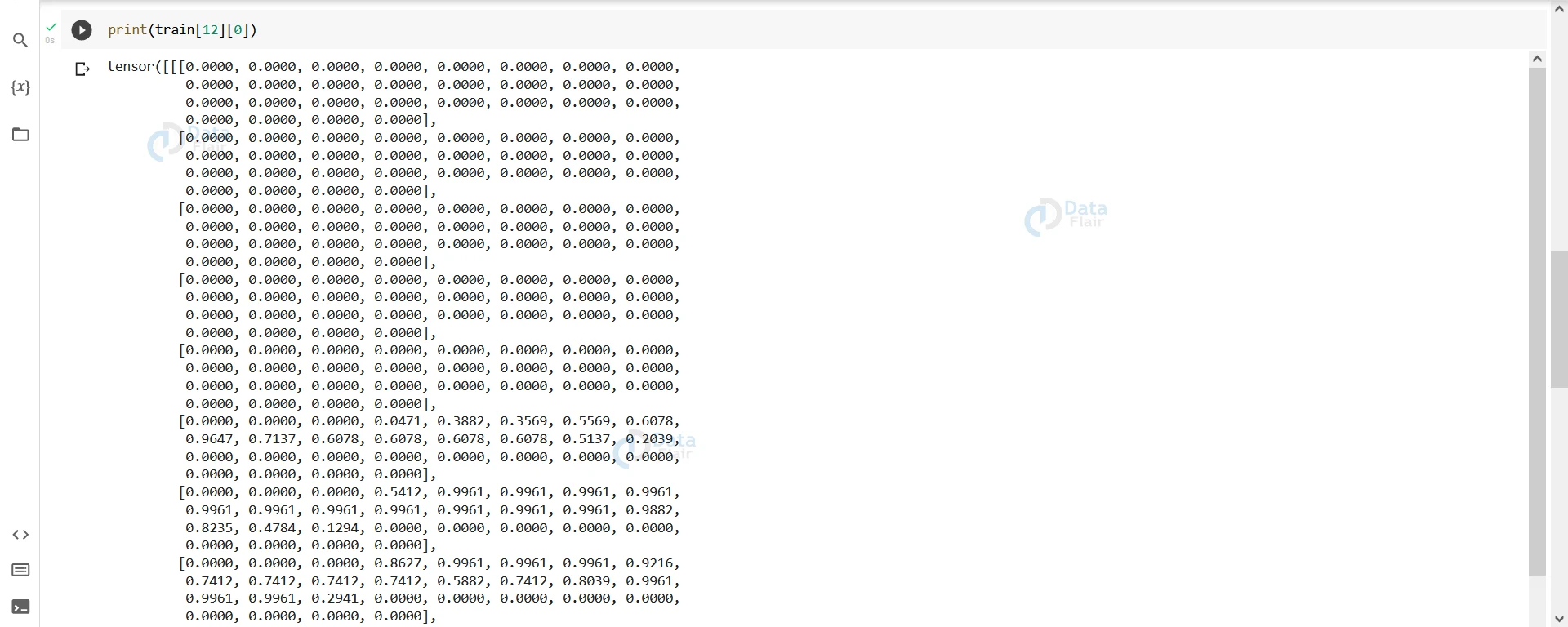
Here, we have printed some random labels of the MNIST dataset. We can also print the tensors representing these labels.

print(train[12][0])

Output

e. Building the Convolutional Model:

Now that we have our data, we can build our convolutional model. First, we will create a forward function that will sequentially implement the convolution layers, followed by activation and pooling layers and finally, the linear layers.

We will also create a function to validate our predictions and print the accuracy later.

class ConvNet(nn.Module):
    def __init__(self):
    	    super(ConvNet,self).__init__()
    
    def forward(self):
      	model=nn.Sequential(nn.Conv2d(1,10,5,padding=2),
                    	nn.ReLU(),
                    	nn.AvgPool2d(2,stride=2),
                   	 
                    	nn.Conv2d(10,20,5,padding=0),
                    	nn.ReLU(),
                    	nn.AvgPool2d(2,stride=2),
                   	 
                    	nn.Flatten(),
                    	nn.Linear(500,250),
                    	nn.ReLU(),
                    	nn.Linear(250,100),
                    	nn.ReLU(),
                    	nn.Linear(100,10)
                   	)
    	     return model
    
    
    def validate(self,model,data):
    	    total=0
    	    correct=0
    	    for i,(images,labels) in enumerate(data):
        	    x=model(images)
        	    value,pred=torch.max(x,1)
        	    total+=x.size(0)
        	    correct+=torch.sum(pred==labels)
    
    
    	    return correct/total

f. Training the model:

Before training our model, we have to specify the device and the number of epochs we want to use. Also, to use our model, we must create an instance of it.

device=torch.device("cpu")
epoch=10
cnn_model=ConvNet()


Finally we will train our model.
cnn=cnn_model.forward().to(device)
cel=nn.CrossEntropyLoss()
optimizer=optim.Adam(cnn.parameters(),lr=0.01)
    
for epoch in range(epoch):
  for i,(images,labels) in enumerate(trainset):
    	    images=images.to(device)
    	    labels=labels.to(device)
    	    optimizer.zero_grad()
    	    pred=cnn(images)
    	    loss=cel(pred,labels)
    	    loss.backward()
    	    optimizer.step()
       	 
  accuracy=cnn_model.validate(cnn,testset)
  print(epoch,accuracy)

It will take a while to train the model.

Output–

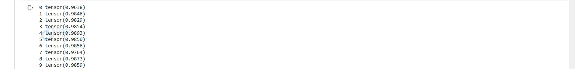
We have successfully implemented a CNN model and achieved remarkable accuracy. It was preprocessed data. Therefore we got such accuracy. However, in practical scenarios, we might not get such accuracy.

Summary

PyTorch makes it very convenient for us to implement a Convolutional Neural Network by providing several convolutional layers. These models are mostly used for image-related applications. However, we can also use it for Natural Language Processing, which was previously tackled by RNN, with even better results than RNNs.
Also, many pre-trained models trained on popular datasets are available on the web. Some of them are -VGG19, ResNet50, GoogleNet. We can play around with these models to predict outputs on new inputs and get a feel of the working of a sophisticated convolutional network.