Pivot Table in Excel

In this blog, we will discuss how to form a pivot table in MS-Excel, what a pivot table is and what are the features in a pivot table.

What is Pivot table in Excel?

Pivot table is a table where the report is generated for the data records in the spreadsheet. It consolidates the data and finds the counts, averages, sums, and other statistics in which the attributes can be grouped in order to draw a meaningful interpretation. It is one of the data pre-processing techniques.

Pivot tables are widely used to make a quick analysis of the data, derive some conclusions and decisions from it.

Why Excel pivot table?

Pivot table is widely encouraged because the table is being formed quickly and it’s flexible whereas the other tables are static. Unlike normal tables, pivot tables are changeable at any point and if the dataset is being updated then pivot table automatically updates the table.

Things you should consider before forming a pivot table

• There should be no blank row or column.
•  Make sure there is no unnecessary cell filled up in the dataset itself.

For example Total at the end of a column in the dataset.

How to create a pivot table in Excel?

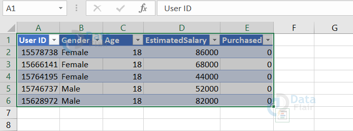
1: To form a pivot table, you should have a dataset.

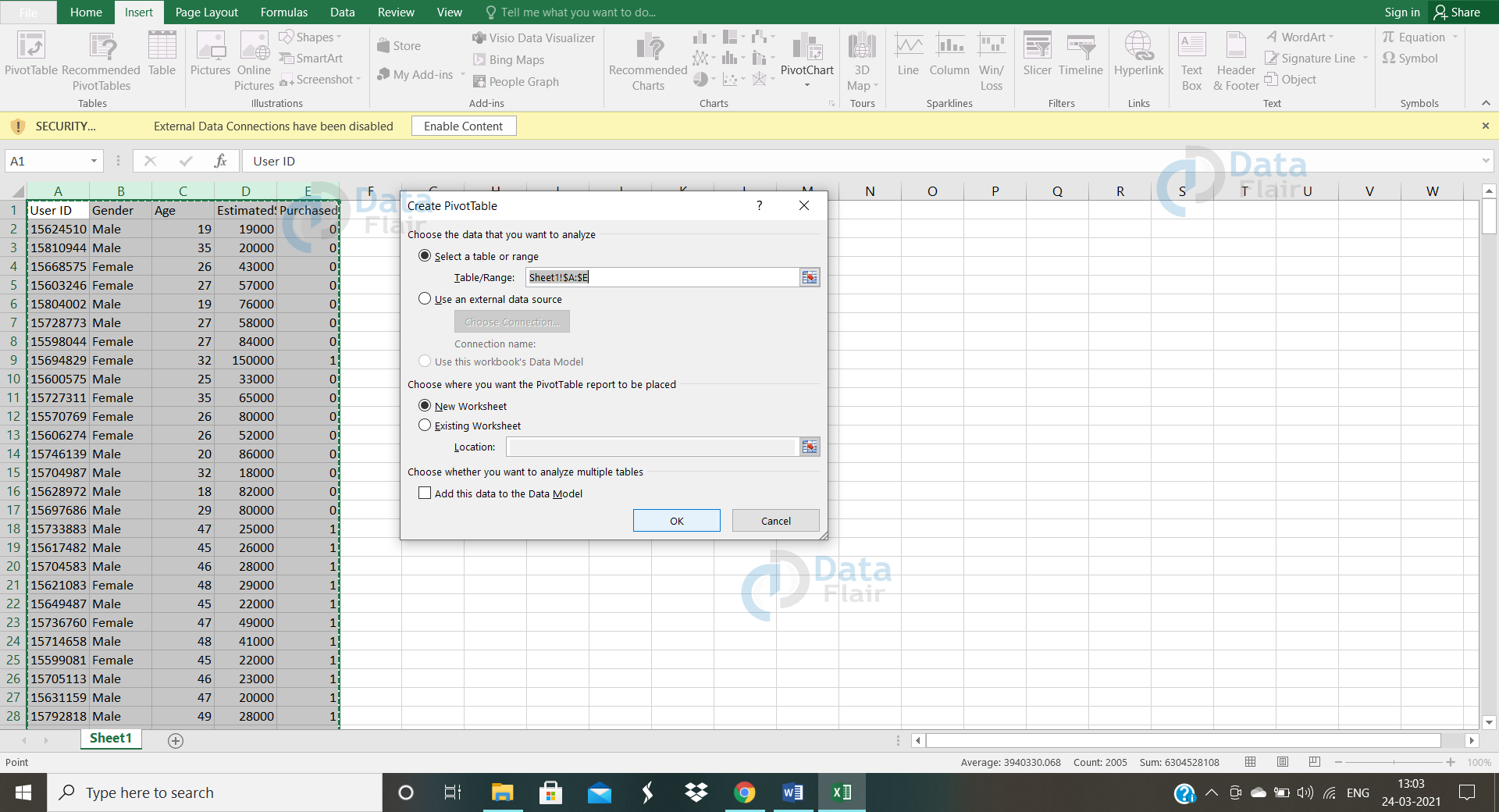
2: After fetching the dataset, select the data range to which the pivot table action should be applied.

3: Click on the INSERT tab and choose the PIVOT TABLE label which is on the left side. Then, click on the “OK” button in the box once you have chosen where your pivot table should appear.

Note: It’s better to have your pivot table in the new worksheet rather than in the existing worksheet.

4: If you have clicked on “New worksheet”, a blank spreadsheet will be automated with the fields besides.

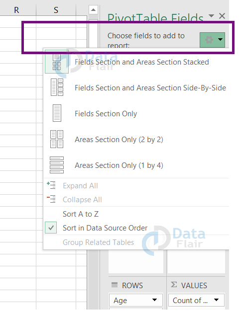
5: You can choose the fields of your data from the pivot table fields. You can drag the fields and drop it in the areas at filters, columns, rows, values as according to convenience.

Note: If you want to change the way the field appears, then you can click on the dropdown near the settings icon and choose any one among the options provided below.

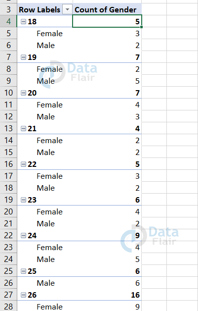
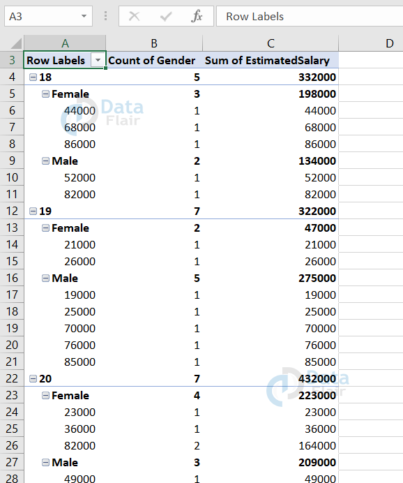
Example: For the sample dataset, we are going to count the number of people in the same age classified by their gender.

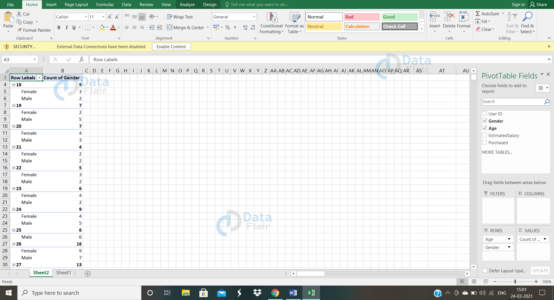
Interpretation:

From the dataset, we can observe that there are totally 3 females and 2 males which resulted as the sum of 5 beside the age 18.

These were the steps to form a simple pivot table.

Change in Summary Calculation

Now, we will see how to change the summary calculations at our convenience. In order to do that, follow the steps:

1: Right-click on the pivot table.

2: Choose the “value field settings” option.

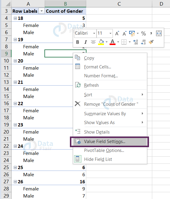
3: Choose the function you want to perform.

For our sample, we are going to sum the estimated salary according to their gender.

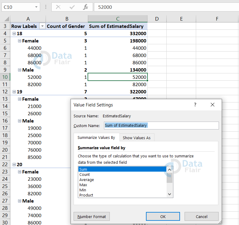
Once you click on the sum, the calculation takes place and it’s viewed as one of the columns in the table.

Customizing the fields to calculate

In the pivot table, we can add columns for calculation purposes. In order to do that, follow the steps:

1: Click on the Analyze tab from the menu.

2: Choose Fields, Items & sets option from the ribbon.

3: Click on the “calculated field..”option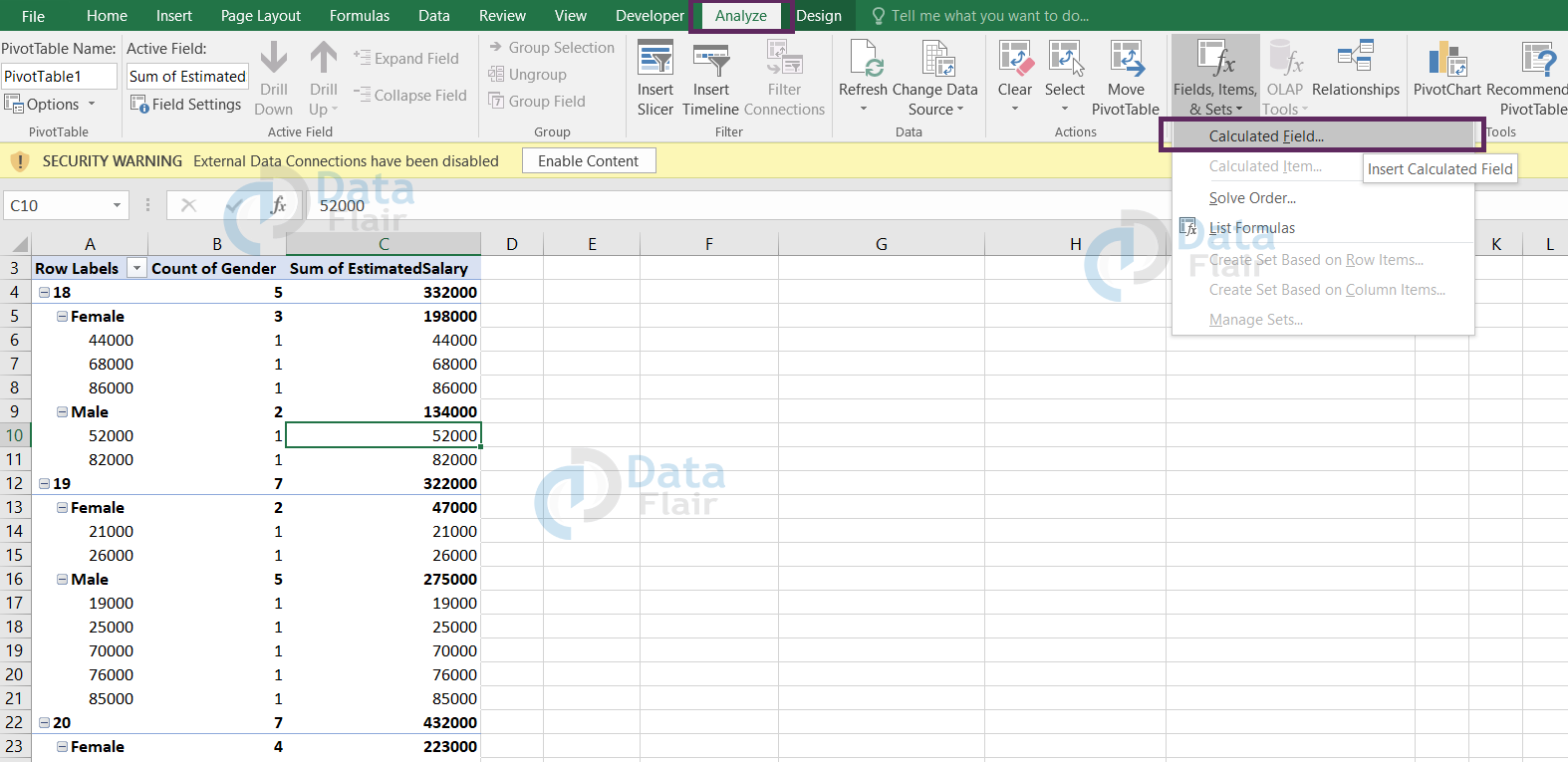

4: A box appears asking about the heading and the formula type.

Note: In the formula type, you will enter the required calculation you wanted to perform in the table.

5: To fill the formula, double click on the required fields and then it is automatically viewed in the formula label option.

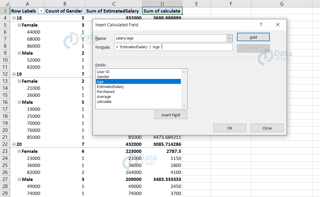
6: Once you press ok, the column will be visible in the pivot table.

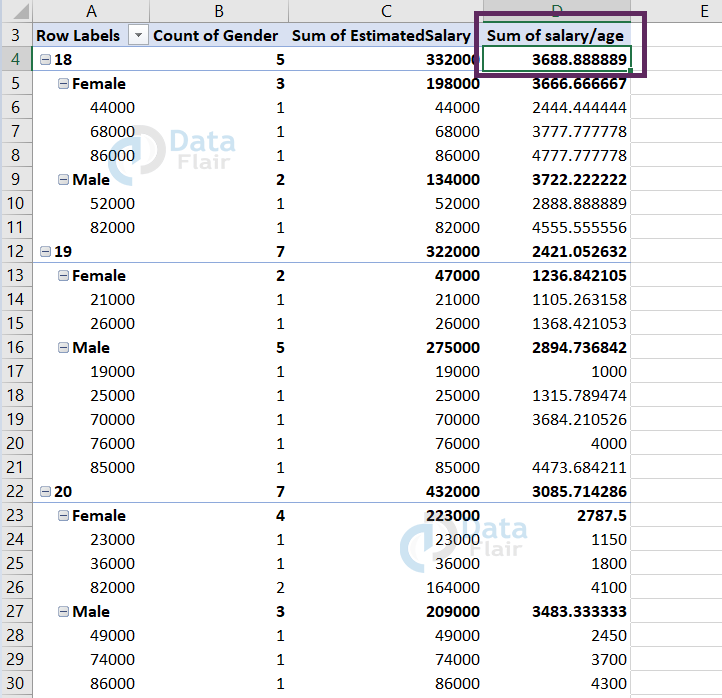
From the sample, we can observe that the custom calculation that we entered is now visible as one of the columns in the pivot table.

There is also an advanced method of forming the pivot table. It is available in new versions of excel. It is also simple and quick to implement.

1: Select the data to which recommended pivot tables has to be applied.

2: Click on the INSERT tab and choose the recommended pivot tables.

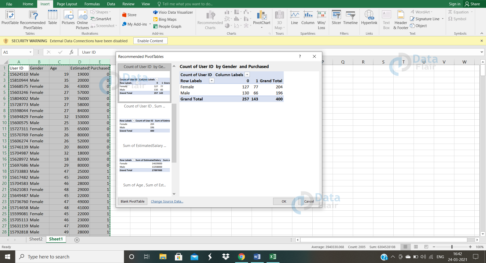
And then the recommended pivot tables show the number of tables the dataset could form for better interpretation of the data.

3: Choose the recommended table if it’s required and click on the OK button. The pivot table will be generated in the new worksheet.

Note: If you wanted to form your customised pivot table, then click on the blank pivot table button.

Once it is being clicked, a blank pivot table appears and then you can proceed with the above steps of the simple pivot table.

Now you may be wondering how those fields are being formed?

When you’re doubtful with the statistics it has performed then, just double click on the cell and then the new worksheet will be formed explaining how it has accumulated the sum or how the analysis has been done.

A demo has been demonstrated below:

Example: I wanted to check how the table has decided its 5. So, I just double-clicked on 5.

Hence, this is how a pivot table is being formed.

Advanced features of pivot table in Excel

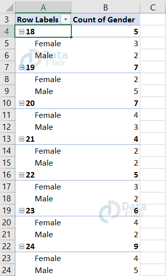
The ‘-’ symbol near the number shows that it has expanded its classification, whereas when we click on it, it changes to ‘+’ symbol with the details hiding.

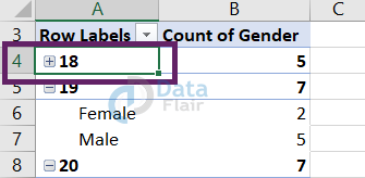
For example: Look at the changes in cell A4 after clicking on the ‘–’ symbol. It has been converted to the ‘+’ symbol by hiding the counts of male and female individually.

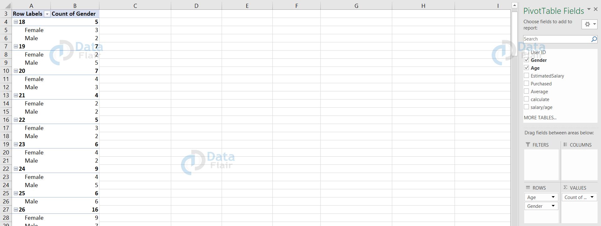
We can also change the table headers as per the requirement. To do this, click on the cell and change it in the formula bar. Hope, you have seen that “row labels” have been changed to “Age”.

The other super special feature is slicer in the pivot table.

First of all, let’s understand what a slicer is?

Slicer is also the same as filtering but instead of using a drop-down menu, we can set up the slicer beside itself and work upon it. The other advantage of a slicer is that it can be connected with one or more pivot tables.

 To set up a slicer to a pivot table, click on the INSERT tab and choose the slicer option.

Once you click, you will see a box in the spreadsheet with the attributes of the dataset.

Choose the attributes to which slicers have to be applied and then click “OK”.

Example: For this dataset, I am going to click on the attribute “gender” and let’s see how it works.

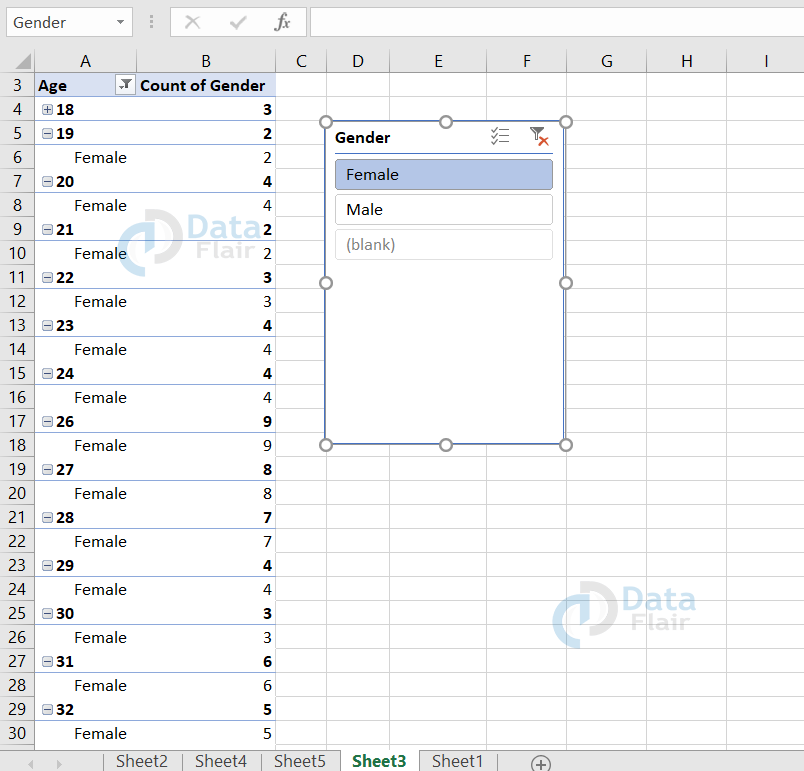
In this slicer, I have chosen only the female and that’s why the table contains only the female count in it.

If we wanted to filter for more than one variable, then you can click on multiple-choice option and choose whichever options you require in the slicer.

Modifying the pivot table in Excel

In a pivot table, adding other columns is also possible. To do this, follow the steps:

1: Click on the pivot table.

2: You will find the fields and variables on the right side of the sheet.

3: Click on the variable and drop it in the fields as per convenience.

Let’s look at a sample:

Now, we wanted to add another attribute to the table. Here, we wanted to view the sum of estimated salaries also. So in order to add that to the table, check the box for the estimated salary and drop it in columns, values fields.

Once we follow the above steps, the column is being viewed in the pivot table. Hence, we can modify a pivot table even after forming it.

Deletion of columns in Excel

Now, let’s see how to delete a column in the pivot table. In order to delete a column from the pivot table, follow the steps:

1: Right-click on the column.

2: Choose the remove “column” option from the list.

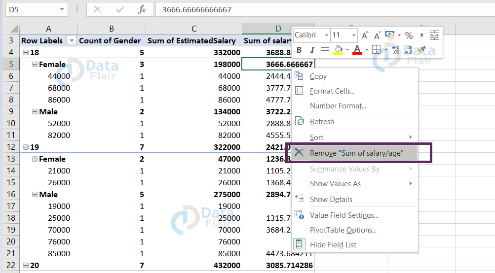
The column will be deleted from the pivot table.
In this sample, we wanted to delete the salary/age column. After following the steps, the table will look like:

Customizing the table in MS Excel

Using filters, we can choose the fields we have to focus on. In order to do that, follow the steps:

1: Click on the arrow mark in the first variable.

2: Deselect the select all option.

3: Choose the required fields alone.

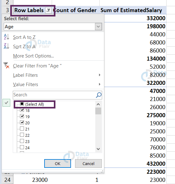
4: Press OK.

In this sample, we are willing to look at the fields of 18,19 and 20 alone. Hence, we have selected only those fields in the option.

We can also sort the data records in the table. In order to sort the data for your convenience, follow the steps:

1: Right-click anywhere on the table.

2: Choose the sort and select either sort from largest to smallest or the sort from smallest to largest.

The table sorts it accordingly.

Let’s look at a sample to see how it sorts the data records.

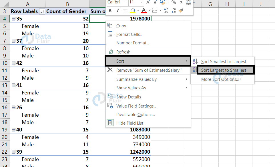
In this sample, we wanted to sort it from largest to smallest. So, we have chosen the sort largest to smallest option.

The dataset now appears like this:

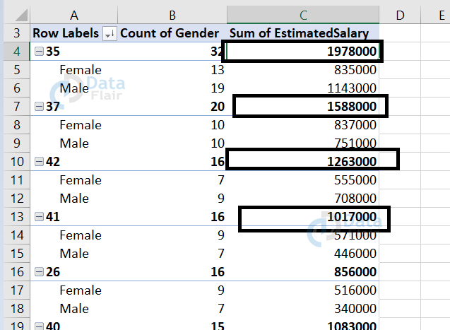
Hope, you can observe that the values are in descending order.

This is one type of sorting and there is also another way to apply sorting to the table. In order to do that, follow the steps.

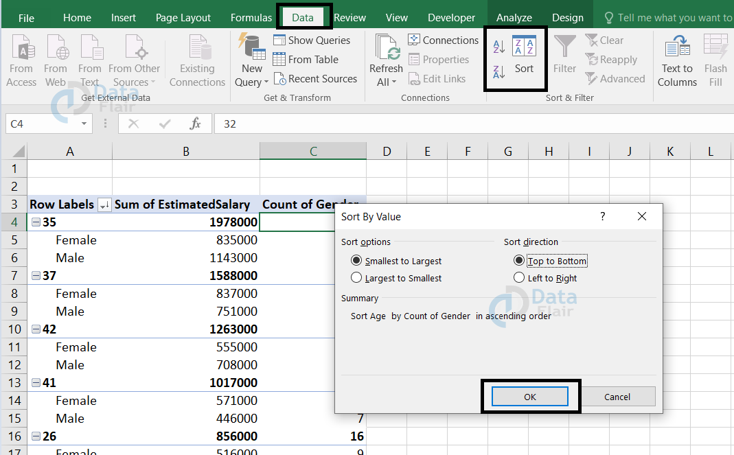
1: Place the cursor anywhere on the pivot table.

2: Click on the Data tab.

3: Click on the sort option.

Note: A box appears with radio button choices and with a summary. So, this can be helpful to you when you aren’t sure about which type of sorting to apply. You can either apply row-wise sorting or column -wise sorting.

When you choose the sort options and sort direction, the summary appears as per your dataset attributes and how it will perform. This is another way to apply sorting to the pivot table.

Creating Excel Pivot table for multiple sheet data

In order to create a single pivot table for multiple sheets data, follow the steps:

1: Press alt+D.

2: Press p. A box appears like this.

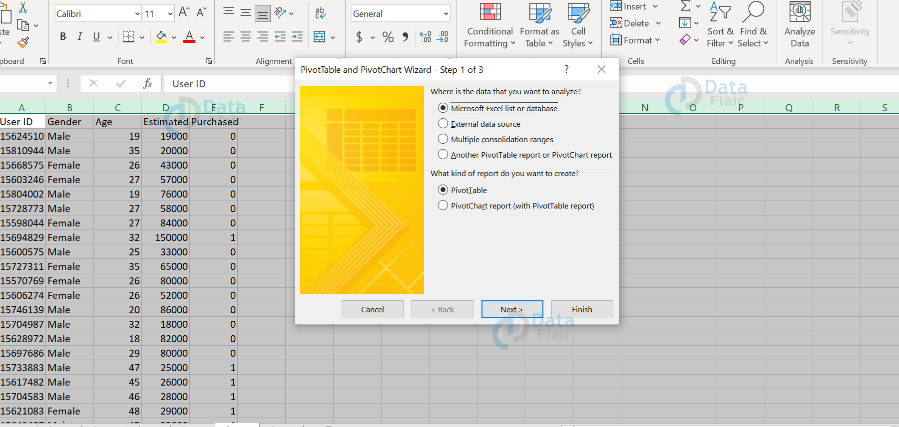
3: Choose the third option i.e., “Multiple consolidation ranges”.

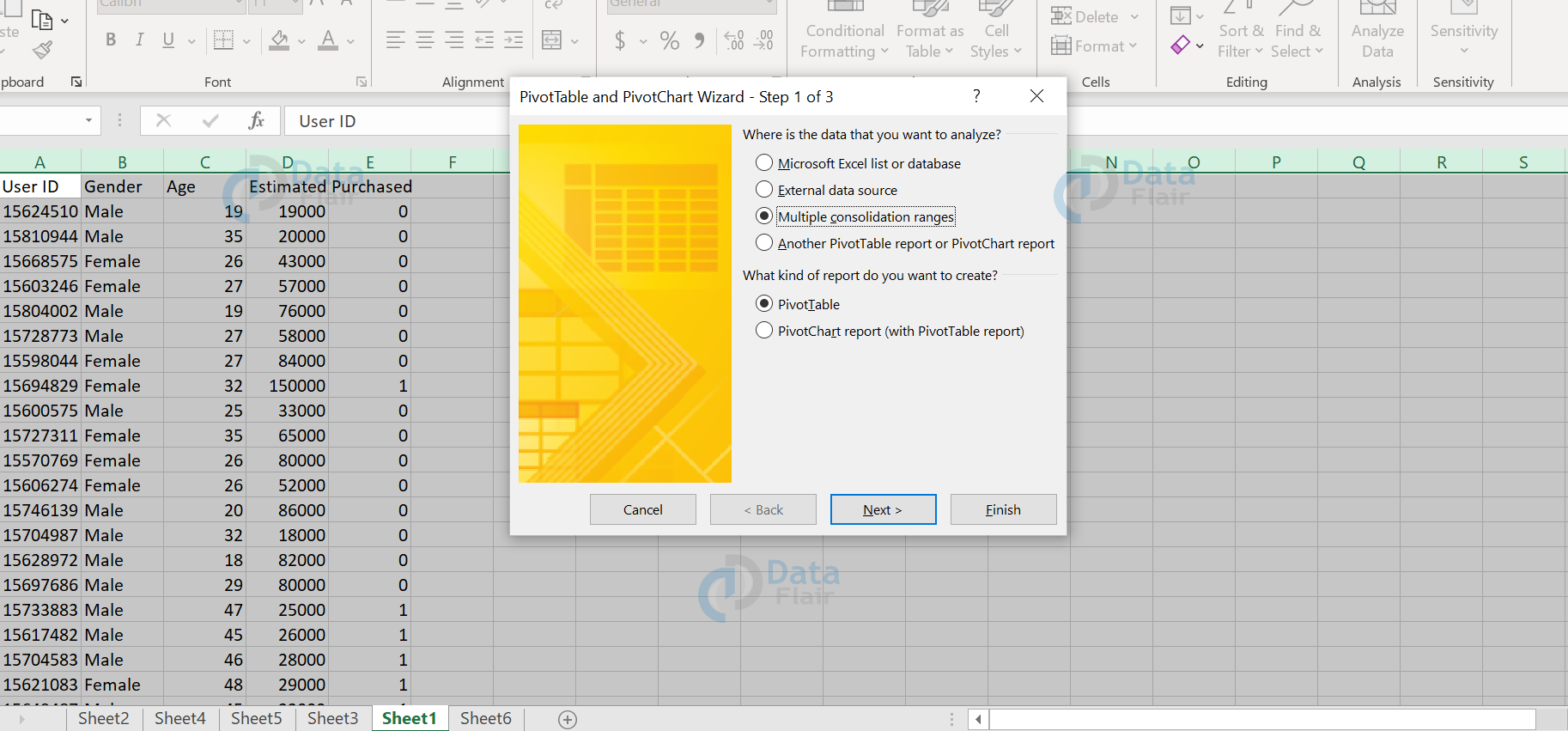
4: Press on the next option.

5: Now choose “I will create the page fields” option.

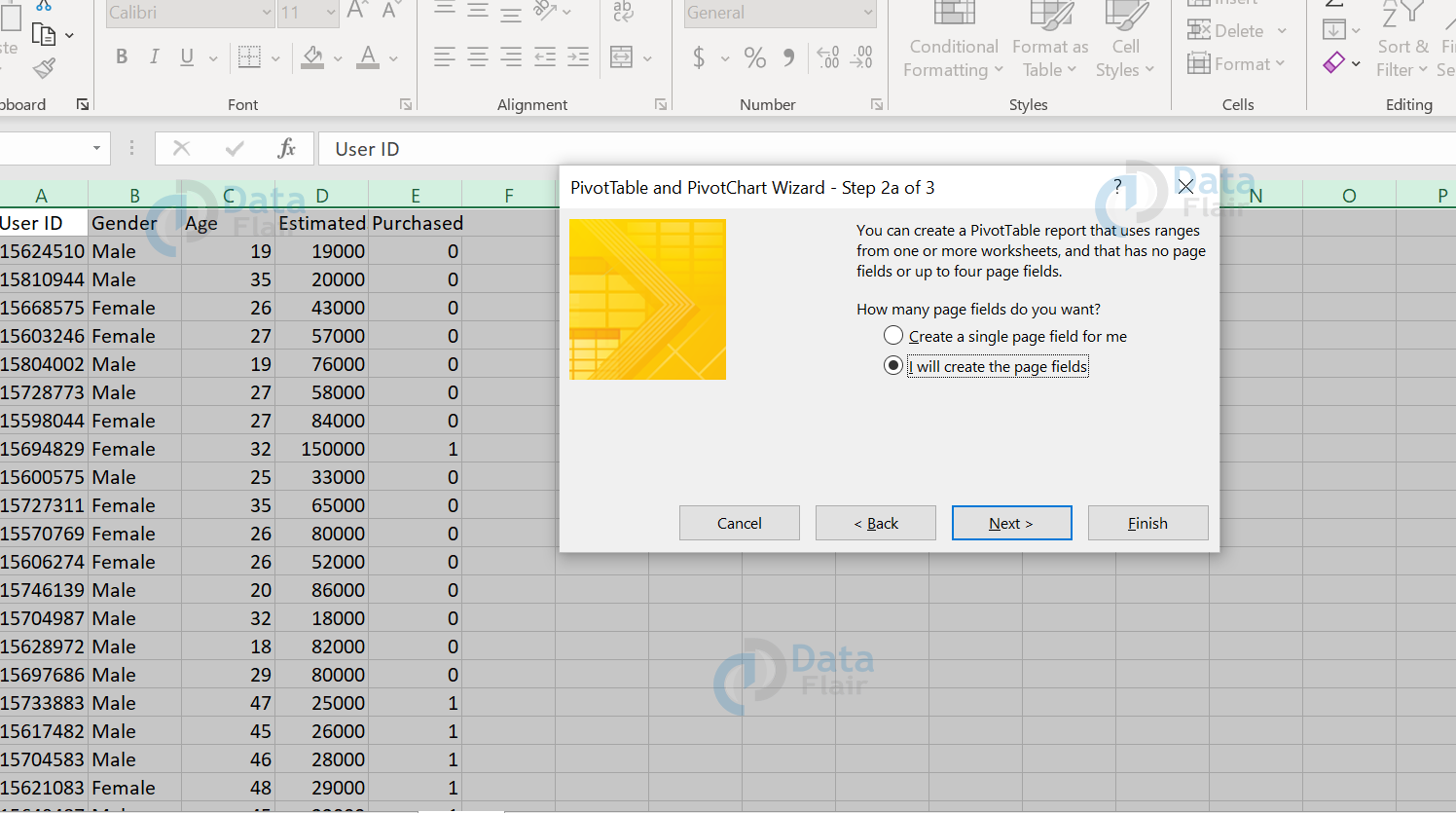
6: Next, choose the range of the sheet. After adding a sheet range, click on the add button to add the next sheet range.

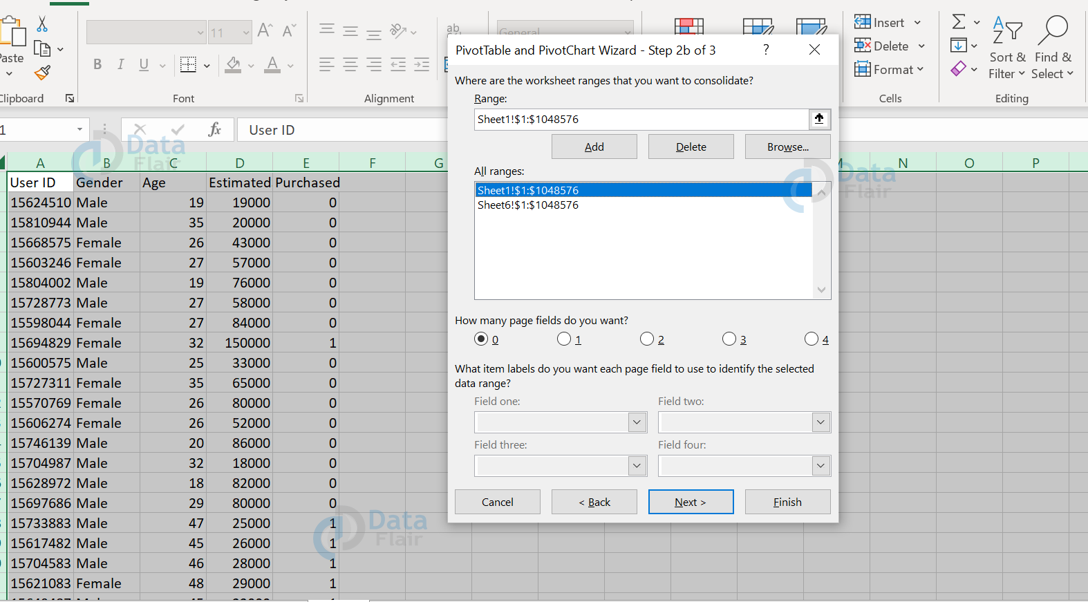
7: Click on the Next option and press Finish option.

Thus, the pivot table for the multiple sheet datasets will be visible now.

2D pivot tables in Excel

Two-dimensional pivot tables are also known as 2d pivot tables. It is also like a simple pivot table but in this 2d pivot table, we will have the attributes in both row and column fields and that is why it is being termed as a 2D pivot table.

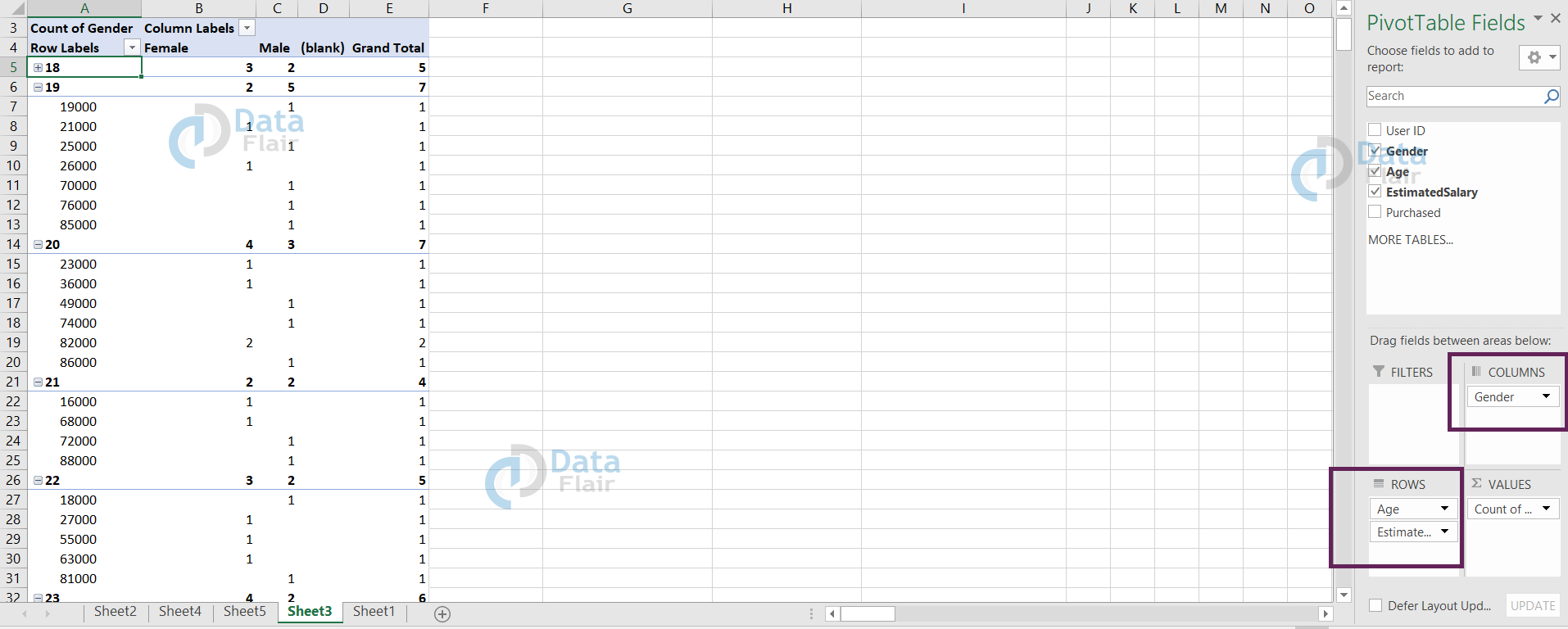
For the sample dataset, we have generated the report for gender and estimated salary which is a 2-Dimensional pivot table.

Pivot Charts in Excel

Charts are being used for better understanding of the dataset and we can also apply charts for the pivot table. This helps us to draw more insights of the dataset.

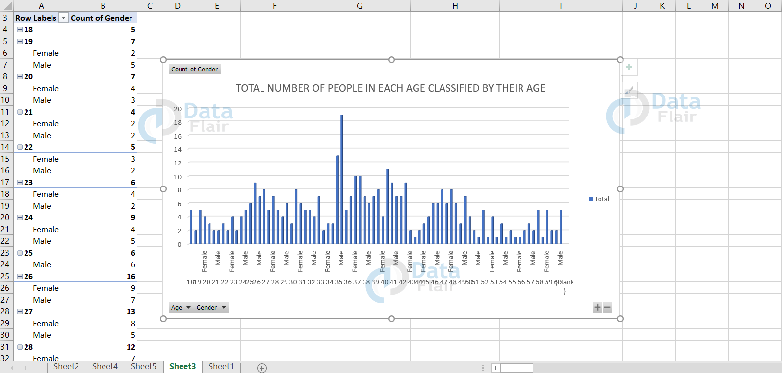
For the sample dataset, we have generated the pivot table summary and a pictorial representation of the pivot table. It represents the count of females and males in each age.

Deleting Pivot table in Excel

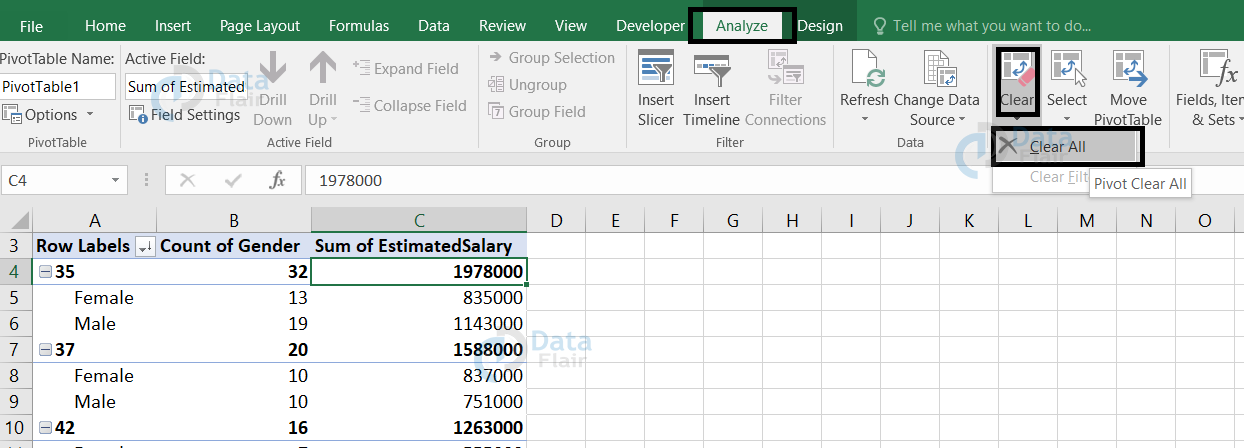
We can also delete a pivot table in a worksheet. In order to delete a pivot table, follow the steps:

1: Keep the cursor on any cell on the table.

2: Choose to analyze tab and click on clear.

3: You will see an option “clear all”. Just click on it and the table will be removed from the worksheet.

Summary

Pivot table feature in MS Excel is a very powerful and useful tool. In no time, it can summarize any amount of data. It helps in summarizing the dataset to draw out some conclusions. It helps us to visualize the dataset using pivot charts.