Optimising Model Parameters Using PyTorch

After a model is built, we train it using our dataset. To do so, we must calculate the loss and optimise the model accordingly. Optimising the parameters is the essential step of the training process because getting the correct (not exact) weights is why we take the burden of dealing with such a huge dataset in the first place. In this article we will see Optimising Model Parameters Using PyTorch.

How Do We Optimise a Model?

When a batch of the dataset passes through the network and outputs are computed, we compare it to the given label of each input and calculate the loss. Then we calculate the gradient of the loss for each parameter (in this case, weights) and try to adjust it to reduce the error. After we have done this with diverse and significant training examples, the weights get generalised, and we say that the training process is complete. There are many ways we can optimise our network, the most popular method being gradient descent.

What is Gradient Descent?

Let J(Ө) be the loss function and Өj the parameter we want to optimise. We update Өj as follows:

Өj:= Өj - α ∂J(Ө) /∂Өj

Where ∂J(Ө) /∂Өj is the gradient of the loss with respect to the parameter under consideration, and α is the learning rate.

We are basically choosing a point at the loss curve and finding the gradient with respect to a parameter. Depending on the gradient, we are moving a small step of size α in a direction where the loss minimises. The next time we do this step, we take the last step’s final point as the starting point and again calculate the gradient and repeat the process. After a few steps depending on the learning rate, we finally reach an optimum value where the loss is minimised.

Using PyTorch to Optimise the Model Parameters

PyTorch has a package called optim, which makes it easy for us to optimise the parameters during the training process. To use it, all we have to do is create an object of torch.optim specifying the model parameters and the learning rate.

After we have made the model, we import torch.optim and then create an object of optim:

import torch.optim as optim
optimiser=optim.SGD(net.parameters(),lr=0.01)

In this example, we are using Stochastic Gradient Descent to optimise our model. There are other optimisers too which can be used like Adam, ASGD etc. The arguments we have passed are the learning rate and net.parameters(), where the net is an instance of the class of our model.

The main role of our optimiser is in the training loop.

for i in range(epoch):
    optimiser.zero_grad()
    output = model(input)
    loss = loss_fn(output, target)
    loss.backward()
    optimiser.step()

In the second line, we call the optimiser.zero_grad to set all the gradients of the network parameters to zero after going through the network once because if we don’t do it, then the gradients of the previous iteration will add up to the gradients of the present iteration and give wrong results.

Then we find the output of one iteration and the loss. After that, we backpropagate through our network to store the gradients of the parameters and then call the optimiser.step() to optimise the model. It is as simple as that. Our model is now optimised for the current step, and we may move to the next iteration.

Example (FASHION MNIST classification)

a. Importing the required libraries

import torch
import torchvision
import torch.nn as nn
import torch.optim as optim
from torchvision import transforms,datasets
import torch.nn.functional as F
import matplotlib
import matplotlib.pyplot as plt

b. Preparing the dataset

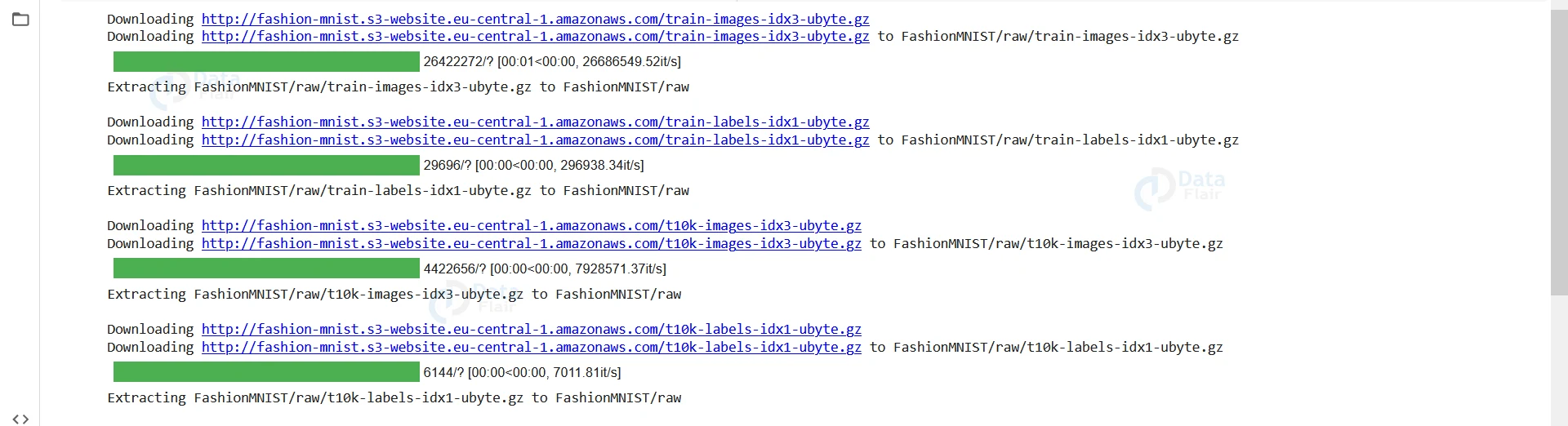
train=datasets.FashionMNIST("", train=True,download=True,transform=transforms.Compose([transforms.ToTensor()]))
test=datasets.FashionMNIST("", train=False,download=True,transform=transforms.Compose([transforms.ToTensor()]))
 
trainset=torch.utils.data.DataLoader(train,batch_size=64,shuffle=True)
testset=torch.utils.data.DataLoader(test,batch_size=64,shuffle=True)

Output-

c. Building the Neural Network

class ConvNet(nn.Module):
    def __init__(self):
            super(ConvNet,self).__init__()
            
            self.model=nn.Sequential(nn.Conv2d(1,10,5,padding=2),
                        nn.ReLU(),
                        nn.AvgPool2d(2,stride=2),
                        
                        nn.Conv2d(10,20,5,padding=0),
                        nn.ReLU(),
                        nn.AvgPool2d(2,stride=2),
                        
                        nn.Flatten(),
                        nn.Linear(500,250),
                        nn.ReLU(),
                        nn.Linear(250,100),
                        nn.ReLU(),
                        nn.Linear(100,10)
                       )
    
    
    
    
    
    def forward(self, x):
      
        fitt = self.model(x)
        return fitt

d. Initialising the Hyperparameters

Hyperparameters are adjustable parameters that alter, or rather control, the training process of the model.

l_rate:( Learning rate) – It determines the speed at which the model moves down to the optimum solution in the learning rate.

Batch_size – Determines the number of samples that are fed to the model at once for training.

Optimiser – This is where we select the optimiser we need for the given task.

l_rate=0.0001
batch_size=64

epoch=10
cnn_model=ConvNet()
 
 
cel=nn.CrossEntropyLoss()
optimizer=optim.Adam(cnn_model.parameters(),l_rate)

e. Training loop

def training(dataloader, model, loss_fn, optimizer):
    size = len(dataloader.dataset)
    for batch, (X, y) in enumerate(dataloader):
        # Compute prediction and loss
        pred = model(X)
        loss = loss_fn(pred, y)
 
        # Backpropagation
        optimizer.zero_grad()
        loss.backward()
        optimizer.step()
 
        if batch % 100 == 0:
            loss, current = loss.item(), batch * len(X)
            print(f"loss: {loss:>7f}  [{current:>5d}/{size:>5d}]")

f. Training the Model

for i in range(epoch):
  print("Epoch",i)
  training(trainset,cnn_model,cel,optimizer)

Output-

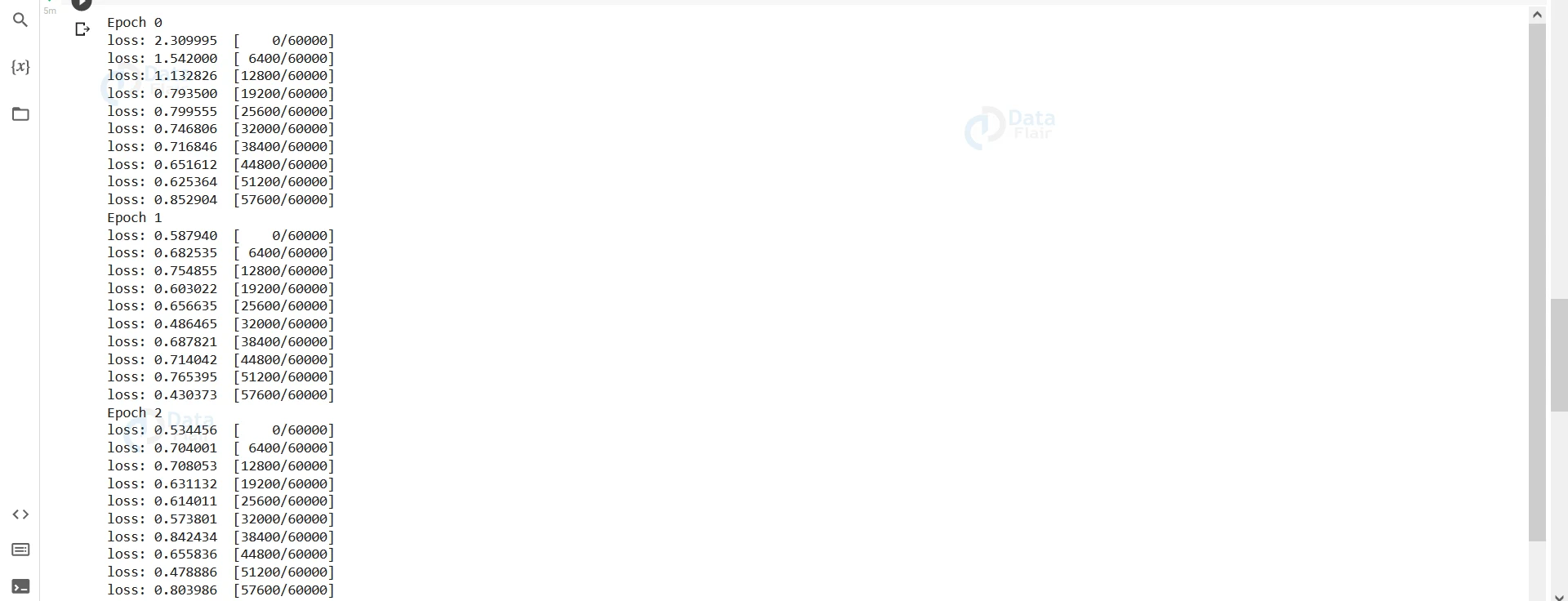
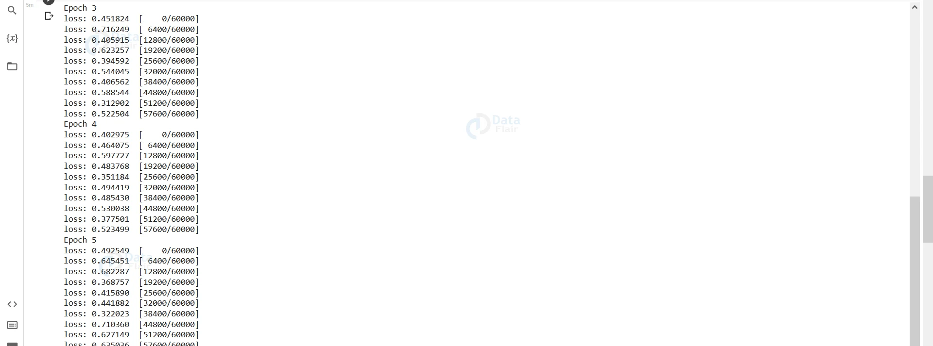
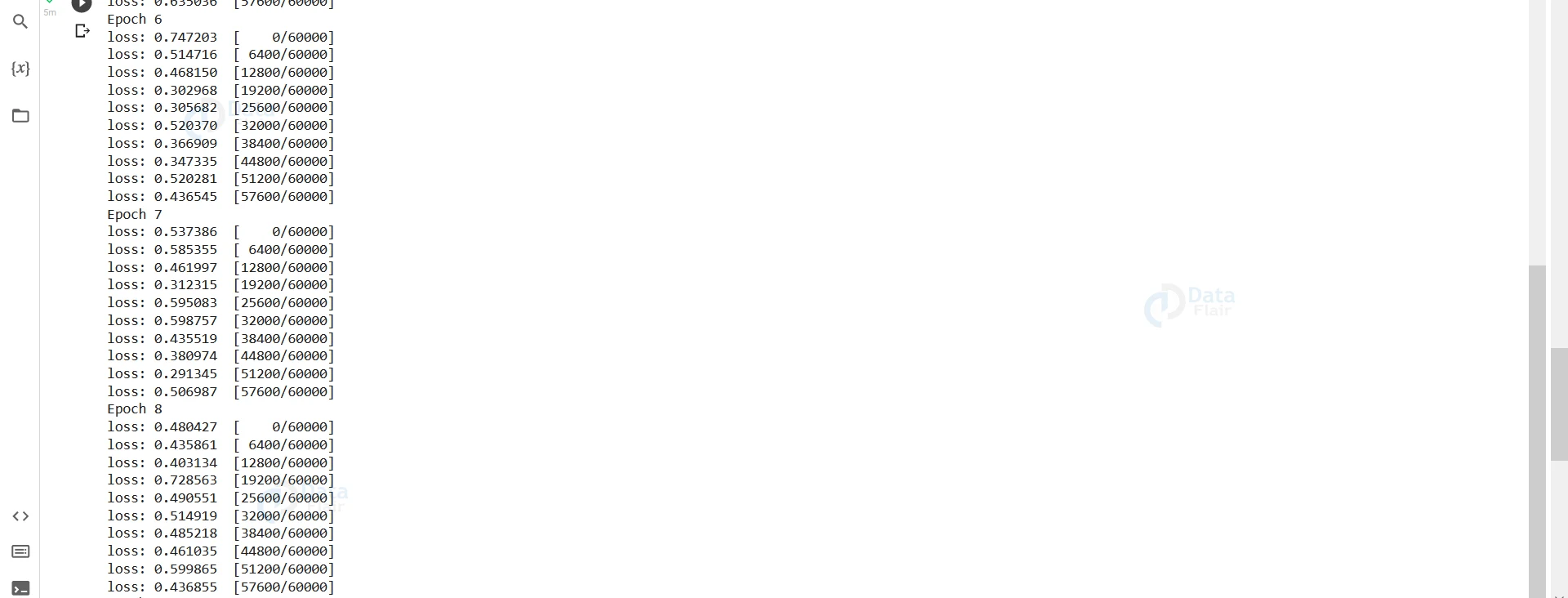
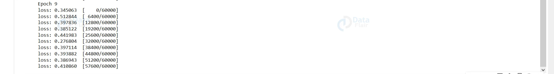
We can see the loss gradually decreasing and then roughly oscillating between a narrow range of values. It indicates that our model’s parameters have reached very close to the minimum of the loss curve, and our model is now optimal.

Important Optimisers in PyTorch:

1. Adadelta

This optimiser implements the Adadelta algorithm, which is a gradient descent algorithm with an adaptive learning rate per dimension.

2. Adagrad

The Adagrad optimiser implements the Adagrad algorithm, which has an adaptive learning rate per component.

3. Adam

The Adam optimiser is a combination of two gradient descent algorithms- Momentum and Root Mean Square Propagation. The momentum algorithm speeds up the descent process based on the exponential weighted average, and the Root Mean Square Propagation method calculates the RMS values instead of the cumulative sum.

4. AdamW

It is a derivative of the Adam optimiser with improved implementation of weight decay.

5. SparseAdam

SparseAdam optimiser is an implementation of Adam optimiser. It is best suited for sparse tensors.

6. Adamax

It is an Adam optimiser with a generalised infinite norm.

7. LBFGS

This optimiser approximates the Broyden–Fletcher–Goldfarb–Shanno algorithm using limited memory.

8. NAdam

It is an Adam optimiser with Nesterov-accelerated adaptive movement estimation.

Summary

PyTorch makes it very easy for us to optimise our neural networks owing to its optim package. All we have to do is import torch.optim, create an object, and in the training loop, call optimiser.zero_grad, loss.backward and optimiser.step in the correct order.